In the last two posts, we explored the theory behind the Jacobian inverse method for solving the inverse kinematics of a system:

Inverse kinematics using the Jacobian inverse, part 1 Inverse kinematics using the Jacobian inverse, part 2

It’s assumed that you’ve either read those posts or already have a good understanding of how the Jacobian inverse method works. As the title suggests, this post has two major goals:

1. To animate the Jacobian inverse method in Python and visualize its limitations.
2. To learn about creating interactive plots in matplotlib.

The end result

This video demonstrates the Jacobian inverse method in action. The dashed circle represents the maximum reach of the arm, which is based on the lengths of all the individual links. We see that it works for any arbitrary number of joints, and we get an idea of how it tracks a moving target when the end effector is made to move at a constant velocity. We also see one of its major drawbacks, which is its instability at singularities—notice how, when the target is outside the reach of the arm, or when the location of the target forces the arm to straighten out, the joint angles change suddenly and erratically. There are several alternatives and improvements to the Jacobian inverse method that address these issues, but we won’t get into those in this post. Instead, we’ll see how to produce the animations from the video in Python.

The code, part 1

We will create two files, RobotArm.py and jacobianInverse.py, which you can find on Github.

First, create a file named RobotArm.py, or get it from the Github link above.

 1
 2
 3
 4
 5
 6
 7
 8
 9
10
11
12
13
14
15
16
17
18
19
20
21
22
23
24
25
26

import numpy as np
import math

class RobotArm2D:
    '''RobotArm2D([xRoot=0, yRoot=0])

        INPUT ARGUMENTS:

        xRoot, yRoot (optional): x and y coordinates of the root joint.
            Both default to 0 if not set.

        INSTANCE VARIABLES:

        thetas: 1D array of joint angles; contains N elements, one per joint.
        joints: 4 x N array of joint coordinates; each column is a vector
            (column 0 is the root joint and column N-1 is the end effector).
        lengths: list of arm link lengths, containing N elements, where
            lengths[0] is the first link and lengths[N-1] is the last link,
            terminating at the end effector.
    '''
    def __init__(self, **kwargs):
        self.xRoot = kwargs.get('xRoot', 0)
        self.yRoot = kwargs.get('yRoot', 0)
        self.thetas = np.array([[]], dtype=np.float)
        self.joints = np.array([[self.xRoot, self.yRoot, 0, 1]], dtype=np.float).T
        self.lengths = []

We start by defining a class, RobotArm2D. This class will contain the joint angles of our robot arm, the Cartesian coordinates of each joint and the end effector, and the length of each link of the arm. Note that, even though our robot arm exists in two dimensions (the XY plane), we’ll use a 3D representation in our code, not only because this will be more generalizable in case we wish to extend our system to three dimensions, but also because it’ll simplify some of the math, namely the use of cross products. Technically, we’re working in 4D—our position vectors contain a dummy fourth coordinate for use with 4×4 transformation matrices, which perform both rotation and translation.

The __init__() method of our class, i.e., the constructor, has two optional keyword arguments: xRoot and yRoot. These set the location of the root joint, i.e., the first joint of the robot arm. If omitted, they default to 0, which is accomplished by the get() method of the kwargs dictionary. Class instantiation in Python via the __init__() method, as well as functions of a class, are discussed in a little more detail in this blog’s very first post, titled Visualizing K-means clustering in 1D with Python. We also initialize the 1D array thetas, which will contain the joint angle of each joint, and the 2D array joints, in which each column will be a 4D position vector representing the coordinates of a joint. The first column in joints will be the root joint and the last column will be the end effector. Finally, lengths is a list that will contain the length of each link.

28
29
30
31
32
33
34
35
36

def add_revolute_link(self, **kwargs):
    '''add_revolute_link(length[, thetaInit=0])
        Add a revolute joint to the arm with a link whose length is given
        by required argument "length". Optionally, the initial angle
        of the joint can be specified.
    '''
    self.joints = np.append(self.joints, np.array([[0,0,0,1]]).T, axis=1)
    self.lengths.append(kwargs['length'])
    self.thetas = np.append(self.thetas, kwargs.get('thetaInit', 0))

To actually add joints/links to our robot arm, we define the function add_revolute_link(). Note that this allows us to add any arbitrary number of joints. Only the length of the link corresponding to the added joint is required. The initial angle can be specified if desired. The end of the last link is taken to be the end effector.

38
39
40
41
42
43
44
45
46
47
48
49
50

def get_transformation_matrix(self, theta, x, y):
    '''get_transformation_matrix(theta, x, y)
        Returns a 4x4 transformation matrix for a 2D rotation
        and translation. "theta" specifies the rotation. "x"
        and "y" specify the translational offset.
    '''
    transformationMatrix = np.array([
        [math.cos(theta), -math.sin(theta), 0, x],
        [math.sin(theta), math.cos(theta), 0, y],
        [0, 0, 1, 0],
        [0, 0, 0, 1]
        ])
    return transformationMatrix

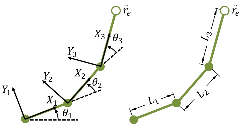
The function get_transformation_matrix() will be used to get 4×4 the transformation matrix corresponding to each joint’s coordinate system. The coordinate systems (and resulting transformation matrices) for the arm are defined as in this previous post:

52
53
54
55
56
57
58
59
60
61
62
63
64
65
66
67
68
69
70

def update_joint_coords(self):
    '''update_joint_coords()
        Recompute x and y coordinates of each joint and end effector.
    '''

    # "T" is a cumulative transformation matrix that is the result of
    # the multiplication of all transformation matrices up to and including
    # the ith joint of the for loop.
    T = self.get_transformation_matrix(
        self.thetas[0].item(), self.xRoot, self.yRoot)
    for i in range(len(self.lengths) - 1):
        T_next = self.get_transformation_matrix(
            self.thetas[i+1], self.lengths[i], 0)
        T = T.dot(T_next)
        self.joints[:,[i+1]] = T.dot(np.array([[0,0,0,1]]).T)

    # Update end effector coordinates.
    endEffectorCoords = np.array([[self.lengths[-1],0,0,1]]).T
    self.joints[:,[-1]] = T.dot(endEffectorCoords)

The function update_joint_coords() updates the coordinates in joints based on the angles in thetas. The function works its way up from root joint to end effector. The transformation matrix for converting coordinates from the root joint coordinate system (“1”) to the global coordinate system (“0”) is \([^0 T_1]\). The coordinates of the root joint, in the first column of joints, are given by xRoot and yRoot and do not change. The transformation matrix to convert from the second joint’s coordinate system (“2”) to the root joint coordinate system (“1”) is \(\left[^1 T_2\right]\). To convert from the second joint system to the global system, these matrices are multiplied: \(\left[ ^0 T_2 \right] = \left[ ^0 T_1 \right] \left[^1 T_2\right]\). This is what lines 63-65 accomplish. For each \(i^{th}\) iteration, the transformation matrix from the previous iteration (which converts from system \(i-1\) to the global system) is multiplied with the transformation matrix from the current iteration (which converts from system \(i\), i.e., the current joint, to system \(i-1\), i.e., the previous joint). For the third joint, lines 63-65 would take the transformation matrix \(\left[ ^0 T_2 \right]\) and multiply it with the transformation matrix for the third joint, \(\left[ ^2 T_3 \right]\): \(\left[ ^0 T_3 \right] = \left[ ^0 T_2 \right] \left[ ^2 T_3 \right]\). In this way, the coordinates of each successive joint are converted to the global coordinate system. Since we’ve defined the end effector to be a vector in the final coordinate system, we multiply that vector by the final transformation matrix to get its coordinates in the global system.

As a side note, observe on line 66 that I enclosed the second index of joints in brackets: self.joints[:,[i+1]]. The reason for this is to preserve the shape of the original array. That bit of code extracts all rows of column i+1 as a two-dimensional, 4×1 array. If, instead, we’d used self.joints[:, i+1], that column would have been “flattened” into a 1D array of 4 elements, potentially leading to incompatibilities when trying to multiply it or add it to other arrays. This is an important thing to note about numpy arrays: an array of shape (4,1) is 2D, and is not the same as an array of shape (4,), which is 1D, even though both arrays contain 4 elements.

72
73
74
75
76
77
78
79
80
81
82
83
84
85
86
87
88

def get_jacobian(self):
    '''get_jacobian()
        Return the 3 x N Jacobian for the current set of joint angles.
    '''

    # Define unit vector "k-hat" pointing along the Z axis.
    kUnitVec = np.array([[0,0,1]], dtype=np.float)

    jacobian = np.zeros((3, len(self.joints[0,:]) - 1), dtype=np.float)
    endEffectorCoords = self.joints[:3,[-1]]

    # Utilize cross product to compute each row of the Jacobian matrix.
    for i in range(len(self.joints[0,:]) - 1):
        currentJointCoords = self.joints[:3,[i]]
        jacobian[:,i] = np.cross(
            kUnitVec, (endEffectorCoords - currentJointCoords).reshape(3,))
    return jacobian

The function get_jacobian() utilizes the cross product to compute each column of the Jacobian matrix (see the previous post for more on this), using the unit vector pointing along the axis of rotation for each joint. In our simplified 2D case, the axis of rotation for every joint points along the \(Z\) axis, i.e., \(\hat{k}\).

90
91

def update_theta(self, deltaTheta):
    self.thetas += deltaTheta.flatten()

The last part of the class is a function, update_theta(), that does exactly what the name suggests. We use the flatten() method of the input array to “flatten” it to a 1D array, so we can add it to the 1D thetas array.

The code, part 2

Now, we’ll utilize the class we just created to animate the algorithm using an interactive plot. Create a file named jacobianInverse.py, or get it on Github.

 1
 2
 3
 4
 5
 6
 7
 8
 9
10
11
12
13
14
15
16

import numpy as np
import math
import matplotlib.pyplot as plt
from RobotArm import *

# Instantiate robot arm class.
Arm = RobotArm2D()

# Add desired number of joints/links to robot arm object.
Arm.add_revolute_link(length=3, thetaInit=math.radians(10))
Arm.add_revolute_link(length=3, thetaInit=math.radians(15))
Arm.add_revolute_link(length=3, thetaInit=math.radians(20))
Arm.update_joint_coords()

# Initialize target coordinates to current end effector position.
target = Arm.joints[:,[-1]]

First, the necessary imports, including the file we created in the last section. We create an instance of the class, add several joints, update the joint coordinates, and initialize the target location to the initial end effector location.

18
19
20
21
22
23

# Initialize plot and line objects for target, end effector, and arm.
fig, ax = plt.subplots(figsize=(5,5))
fig.subplots_adjust(left=0, bottom=0, right=1, top=1)
targetPt, = ax.plot([], [], marker='o', c='r')
endEff, = ax.plot([], [], marker='o', markerfacecolor='w', c='g', lw=2)
armLine, = ax.plot([], [], marker='o', c='g', lw=2)

Next, we create the plot. The argument figsize=(5,5) to plt.subplots() on line 19 sets the figure size; in this case, the goal is simply to set the height and width equal so the figure is square. On line 20, we use subplots_adjust() to position the axis limits at the edges of the figure, so the axes take up the entirety of the plot.

25
26
27
28
29
30
31
32
33
34

# Determine maximum reach of arm.
reach = sum(Arm.lengths)

# Set axis limits based on reach from root joint.
ax.set_xlim(Arm.xRoot - 1.2 * reach, Arm.xRoot + 1.2 * reach)
ax.set_ylim(Arm.yRoot - 1.2 * reach, Arm.yRoot + 1.2 * reach)

# Add dashed circle to plot indicating reach.
circle = plt.Circle((Arm.xRoot, Arm.yRoot), reach, ls='dashed', fill=False)
ax.add_artist(circle)

Now, we compute the reach of the arm and use it to set the axis limits, with some white space at the edges, then plot a circle to indicate the boundaries of the arm’s reach.

36
37
38
39
40
41
42
43

def update_plot():
    '''Update arm and end effector line objects with current x and y
        coordinates from arm object.
    '''
    armLine.set_data(Arm.joints[0,:-1], Arm.joints[1,:-1])
    endEff.set_data(Arm.joints[0,-2::], Arm.joints[1,-2::])

update_plot()

Lines 36-41 define a function, update_plot(), to update the coordinates of the arm and end effector plot objects. Line 43 runs this function to initialize these plot objects with the coordinates from the arm object.

45
46
47
48
49
50
51
52
53
54
55
56
57
58
59
60
61

def move_to_target():
    '''Run Jacobian inverse routine to move end effector toward target.'''
    global Arm, target, reach

    # Set distance to move end effector toward target per algorithm iteration.
    distPerUpdate = 0.02 * reach

    if np.linalg.norm(target - Arm.joints[:,[-1]]) > 0.02 * reach:
        targetVector = (target - Arm.joints[:,[-1]])[:3]
        targetUnitVector = targetVector / np.linalg.norm(targetVector)
        deltaR = distPerUpdate * targetUnitVector
        J = Arm.get_jacobian()
        JInv = np.linalg.pinv(J)
        deltaTheta = JInv.dot(deltaR)
        Arm.update_theta(deltaTheta)
        Arm.update_joint_coords()
        update_plot()

The function move_to_target() actually performs the Jacobian inverse technique, or at least one iteration of it. Line 50 sets how far to move the end effector on each iteration (each update of the arm’s position), as a fraction of the arm’s reach, which essentially scales the arm’s motion to its total length. Basically, this sets the velocity of the end effector, if you think of each iteration as a unit of time, as long as the end effector is farther from the target than the distance specified by line 52 (if it’s closer, then it’s considered sufficiently close, and doesn’t move). On lines 53-54, we get the unit vector in the direction of the target from the end effector. On line 55, we compute \(\Delta \mathbf{r}\), or the vector distance that we’d like the end effector to move (toward the target). The rest of the function computes the Jacobian based on this vector, inverts the Jacobian, computes the change in joint angles, then updates the joint coordinates and the plot with the new arm configuration.

63
64
65
66
67
68
69
70
71
72
73
74
75
76
77
78
79
80
81

# "mode" can be toggled with the Shift key between 1 (click to set
# target location) and -1 (target moves in predefined motion).
mode = 1

def on_button_press(event):
    '''Mouse button press event to set target at the location in the
        plot where the left mouse button is clicked.
    '''
    global target, targetPt
    xClick = event.xdata
    yClick = event.ydata

    # Ensure that the x and y click coordinates are within the axis limits
    # by checking that they are floats.
    if (mode == 1 and event.button == 1 and isinstance(xClick, float)
        and isinstance(yClick, float)):
        targetPt.set_data(xClick, yClick)
        target = np.array([[xClick, yClick, 0, 1]]).T
fig.canvas.mpl_connect('button_press_event', on_button_press)

Now, we arrive at the interactive stuff. First, we define the variable mode, which will assume a value of 1 or -1. Mode 1 signifies that the target will be set manually whenever the user left-clicks somewhere within the plot. Mode -1 signifies that the target will move on its own along a predefined path. This first function, on_button_press(), is responsible for setting the target manually when mode is set to 1.

In matplotlib, event callbacks are defined by a function that takes an event object as an input (whenever an event, like a button click or a key press, occurs, this event object is sent automatically to the function). The event object contains information about the event. In the case of a mouse click, this includes the x and y coordinates, with respect to the plot axes, of the click, which we obtain on lines 72-73. In the conditions on lines 77-78, we check that we’re in the correct mode, that the button equals “1” (“1” denotes the left mouse button), and that the click was within the axis limits (if it wasn’t, the type of the returned coordinates would be None instead of float). Line 81 associates the button press event with the figure via the function on_button_press().

83
84
85
86
87
88
89
90
91
92
93
94
95

# Use "exitFlag" to halt while loop execution and terminate script.
exitFlag = False

def on_key_press(event):
    '''Key press event to stop script execution if Enter is pressed,
        or toggle mode if Shift is pressed.
    '''
    global exitFlag, mode
    if event.key == 'enter':
        exitFlag = True
    elif event.key == 'shift':
        mode *= -1
fig.canvas.mpl_connect('key_press_event', on_key_press)

Next, we do the same thing for a key press event. We’d like the script to terminate if the Enter key is pressed, by setting exitFlag to True. Moreover, we’d like to toggle the mode if the Shift key is pressed. As above, we check whether either of these buttons is pressed and act accordingly. On line 95, we connect the key press event to the figure.

 97
 98
 99
100
101
102
103
104
105
106
107
108
109
110
111
112
113

# Turn on interactive plotting and show plot.
plt.ion()
plt.show()

print('Select plot window and press Shift to toggle mode or press Enter to quit.')

# Variable "t" is used for moving target mode.
t = 0.
while not exitFlag:
    if mode == -1:
        targetX = Arm.xRoot + 1.1 * (math.cos(0.12*t) * reach) * math.cos(t)
        targetY = Arm.yRoot + 1.1 * (math.cos(0.2*t) * reach) * math.sin(t)
        targetPt.set_data(targetX, targetY)
        target = np.array([[targetX, targetY, 0, 1]]).T
        t += 0.025
    move_to_target()
    fig.canvas.get_tk_widget().update()

Finally, after turning on interactive plotting and showing the plot, we employ a while loop to continuously run our move_to_target() function. This way, the arm will track the target any time it moves. If mode is set to -1, the target moves in a pseudo-random fashion, which we accomplish using the continuously changing variable t and, on lines 107-108, a few strategically placed sine and cosine terms. I say “pseudo-random” because, of course, the sines and cosines mean it’s actually cyclical.

The last line, line 113, is required to update the plot after button or key press events. I utilize the figure canvas’s get_tk_widget() method because I’m using the Tkinter backend, so this may be different if you’re using a different backend. Tkinter is the default Python GUI package, and allows us to create GUIs and graphical objects, like plots. Matplotlib is able to work with a variety of different GUI backends, like GTK, Qt, and Wx, to name a few. You can check the GUI backend currently being used with the command plt.get_backend(). You can also list all backends available on your system by importing matplotlib with import matplotlib followed by the command matplotlib.rcsetup.all_backends.

Conclusion

That was a long post, but you now have a functioning script that’ll interactively animate the Jacobian inverse technique. Try playing around with the parameters of the inverse kinematics algorithm to see how it affects the ability of the arm to track a target. For example, set the threshold for the distance between the end effector and target on line 52 of jacobianInverse.py to a value smaller than distPerUpdate and see what happens; since you’d be setting the threshold to a value smaller than the distance the end effector moves during each iteration of the algorithm, the end effector might infinitely overshoot the target without being able to reach it. You can also adjust the value by which t is incremented on line 111 to change the speed of the target in the moving target mode.

Try adding more joints/links to the arm. An easy way to add a lot of joints in one go is with the following code:

for i in range(20):
    Arm.add_revolute_link(length=3)

As for interactive plotting, we’ve just barely scratched the surface. Read the matplotlib documentation on event handling for more on the different types of events. One idea might be to make a plot in which the arm tracks your mouse cursor using the motion_notify_event.