
This post continues from the previous post.
The Jacobian matrix
The Jacobian matrix is effectively the gradient of a vector-valued function, which maps the rate of change of joint angles to the rate of change of the physical location of the end effector. If you're not familiar with multivariable calculus, or if your last calculus class is well in the rear-view, let's look at a simple example: a 2D line.
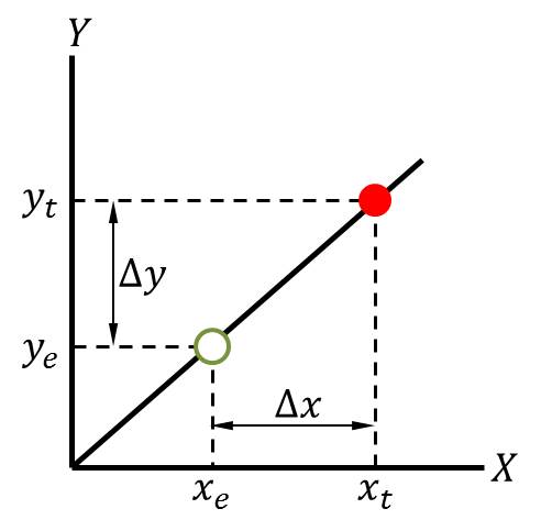
The equation of this line is \(y = mx\), where \(m\) is the slope, i.e., rate of change, of the line. Let's say we're at a point \((x_e, y_e)\) on the line, and we know both \(x_e\) (our horizontal position) and \(y_e\) (our height, or vertical position). We also know the slope of the line, \(m\). Say we'd like to move to a different vertical position, \(y_t\)—however, we don't know the horizontal coordinate \(x_t\) of our target position, i.e., we don't know how far we have to move in the \(x\) direction to achieve our desired change in the \(y\) direction. This gives us the equation:
\[\Delta y = m \Delta x\]
where we know everything except \(\Delta x\). Computing \(\Delta x\) is just a matter of dividing through by \(m\), i.e., multiplying by the inverse of \(m\):
\[m ^{-1} \Delta y = m ^{-1} m \Delta x\]
which is the same as writing:
\[\frac{1}{m} \Delta y = \frac{1}{m} m \Delta x\]
Or, simply:
\[\frac{1}{m} \Delta y = \Delta x\]
The Jacobian inverse method basically does the same thing, except instead of mapping a scalar \(\Delta x\) to a scalar \(\Delta y\) via the slope \(m\), it maps a vector-valued change in joint space \(\mathbf{\Delta} \pmb{\theta}\) to a vector-valued change in physical space \(\mathbf{\Delta r}\) via the Jacobian matrix \(\mathbf{J}\):
\[\mathbf{\Delta r} = \mathbf{J \Delta} \pmb{\theta}\]
So, what does the Jacobian matrix actually look like? For the three-dimensional case, the Jacobian is a \(3 \times n\) matrix, where \(n\) is the number of joints:
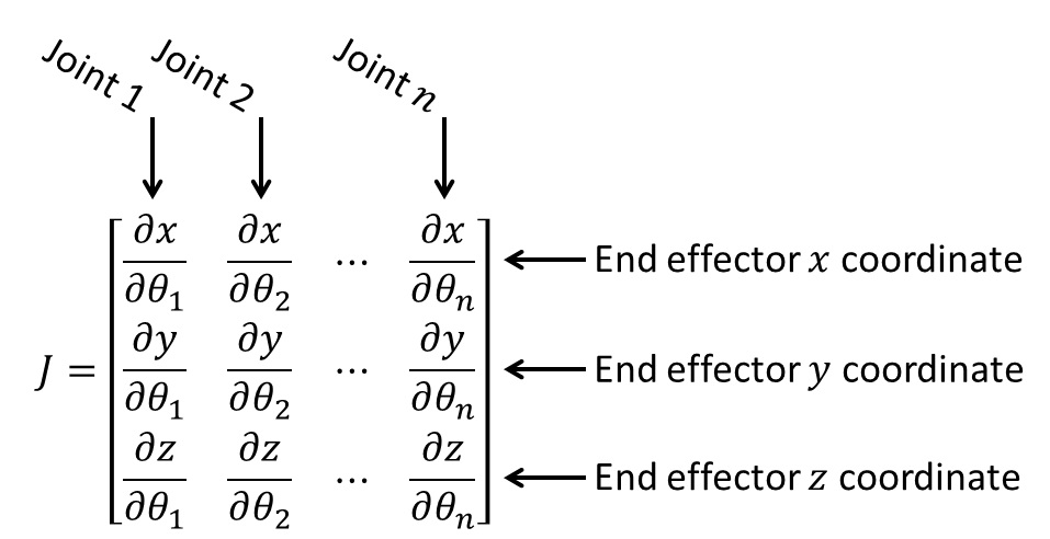
The matrix takes the partial derivative of each component of the end effector position vector with respect to each joint. In other words, each element of the matrix considers how the end effector moves if only one of the joint angles changes. For example, consider the first element (row 1, column 1) of the matrix: \(\frac{\partial x}{\partial \theta_1}\). This element tells us, “if we change the angle of the first joint, \(\theta_1\), while holding the angles of all the other joints constant, how does the \(x\) coordinate of the end effector change?” i.e., what is the rate of change of the end effector \(x\) coordinate with respect to \(\theta_1\)? We do this for every end effector coordinate with respect to every joint. Multiplying the joint angles by this matrix sums the impact of each joint on each end effector coordinate. This is what the equation above, \(\Delta \mathbf{r} = \mathbf{J} \Delta \pmb{\theta}\), does. Writing out the terms in full, as well as the result of the multiplication:
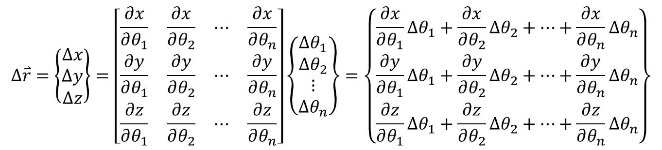
The result says that the overall change in the \(x\) coordinate of the end effector position is the sum of the rate of change of the \(x\) coordinate with respect to \(\theta_1\) times the change in \(\theta_1\) plus the rate of change of the \(x\) coordinate with respect to \(\theta_2\) times the change in \(\theta_2\), and so on for every joint. Same thing for the \(y\) and \(z\) coordinates in the second and third rows, respectively.
Another way of putting this is that we're obtaining the vector tangent to the path of the end effector for each joint, then adding them together:
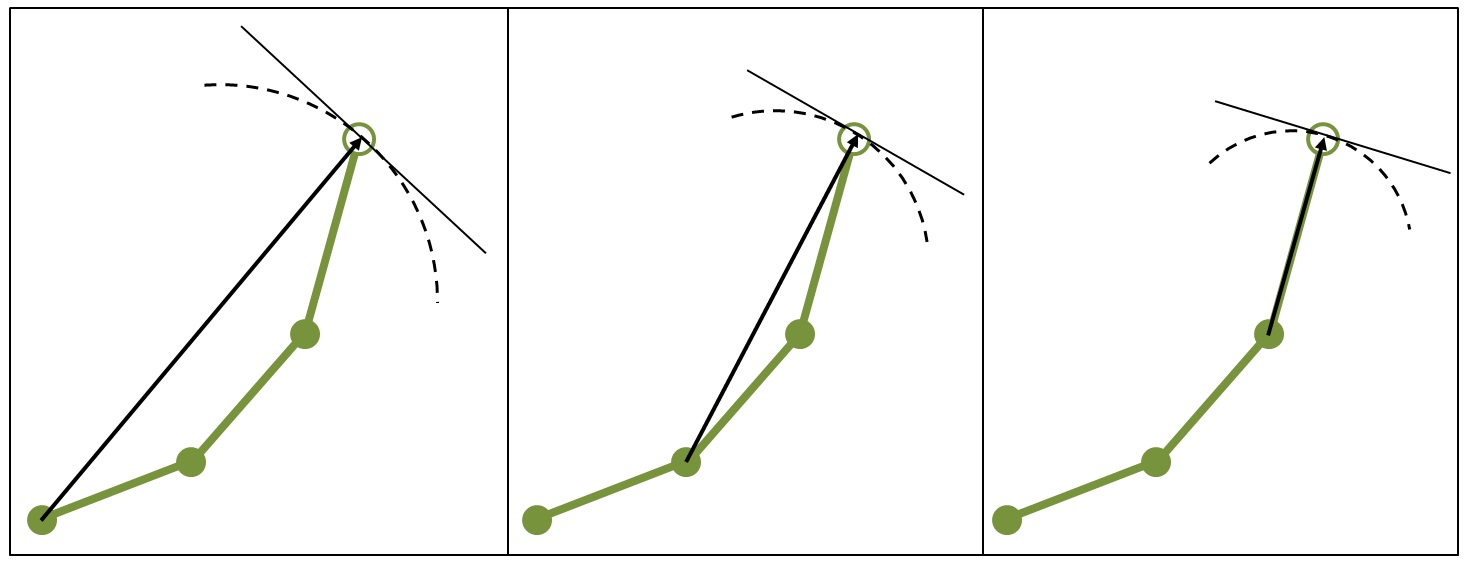
In the figure above, left, the dashed line represents the actual path of the end effector as the first joint rotates, if the other joint angles don't change. The solid line tangent to that arc represents the partial derivative of the end effector with respect to the first joint in the current orientation (at the current set of joint angles), i.e., the instantaneous rate of change in the current orientation. This corresponds to the first column of the Jacobian matrix. Similarly, the next image in the figure shows the path and the rate of change of the end effector with respect to the second joint, which corresponds to the second column of the Jacobian matrix. And so on for every joint, which, in our example, is three joints. In each case, I've drawn a vector from the joint in question to the end effector—this vector represents the radius of the arc representing the path of the end effector (i.e., the dashed line).
Note that, by taking the derivative of the end effector with respect to any joint, we're linearizing the problem. For a given set of joint angles, the Jacobian gives us the instantaneous rate of change—that is, the tangent lines in the figure above. This means that, when we use the Jacobian, we're following the tangent lines—not the dashed lines. For small angular displacements, the tangent lines are an accurate approximation to the dashed lines, but they're inaccurate for large angular displacements (large changes in the joint angles).
How do we actually determine the elements of the Jacobian matrix? One way is to get the end effector coordinates as a function of the joint angles, i.e., \(\mathbf{r_e} = f(\pmb{\theta}) = f(\theta_1, \theta_2, \dots, \theta_n)\), by multiplying the transformation matrices and the coordinates of the end effector in the final coordinate system, which we obtained previously, then take the partial derivative of this function with respect to each joint angle and plug in the joint angles for the current position.
An alternative is to use the cross product, which may be preferable if we're constructing the Jacobian numerically. It turns out that the cross product acts as an infinitesimal rotation generator, which essentially means that we can obtain the vector rate of change of a point, like an end effector, with respect to another point, like a joint, if we know the positions of those points and if we know the axis of rotation. This is given by the following equation:
\[\frac{\partial \mathbf{r_e}}{\partial \theta_j} = \mathbf{a_j} \times (\mathbf{r_e} - \mathbf{r_j})\]
where \(\theta_j\) denotes the angle of the \(j ^{th}\) joint, \(\mathbf{r_j}\) denotes the position of that joint, and \(\mathbf{a_j}\) is a unit vector representing the axis of rotation for that joint.
Refer to the previous figure again. For each joint, the vector from the joint to the end effector is the quantity \((\mathbf{r_e - r_j})\). Then, using the cross product, our definition of the Jacobian matrix can be written as:
\[ \mathbf{J} = \left[ \begin{matrix} \left\{ \mathbf{a_1} \times (\mathbf{r_e - r_{j1}}) \right\}^T & \left\{ \mathbf{a_2} \times (\mathbf{r_e - r_{j2}}) \right\}^T & \dots & \left\{ \mathbf{a_n} \times (\mathbf{r_e - r_{jn}}) \right\}^T \end{matrix} \right] \]
Further, because the robot arm in our example lies entirely in the \(XY\) plane, all of our joints rotate about the \(Z\) axis. Thus, the axis of rotation in our example is always given by the unit vector \(\hat{k}\), which points along the \(Z\) axis.
After constructing the Jacobian matrix, the final step of the Jacobian inverse method, as the name suggests, is to invert the Jacobian matrix. Most of the time, the Jacobian matrix will be non-square, making it non-invertible. Depending on the orientation of the joints, the matrix may also be singular, if one or more joint angles are equal to zero, which also makes it non-invertible. Therefore, the pseudoinverse of the matrix is usually used. Without going into details, the pseudoinverse avoids these problems and always allows an inverse to be computed.
At last, after computing the inverse, we can obtain the joint angles necessary to attain the desired change in end effector position, by multiplying the Jacobian inverse and the change in position:
\[\mathbf{J ^{-1}} \Delta \mathbf{r} = \Delta \pmb{\theta}\]
And there you have it—the Jacobian inverse method for solving the inverse kinematic problem. As mentioned above, the Jacobian provides a linear approximation to the derivative of the position of the end effector. The Jacobian changes as the joint angles change. For small changes in the joint angles, the Jacobian provides an accurate linear approximation to the motion of the end effector, but as the joint angles continue to change, this approximation becomes less accurate. Therefore, the Jacobian inverse is an iterative method. We make a small change to the joint angles, then recompute the Jacobian, and repeat until the end effector is at (or sufficiently close to) the target position.
Final notes
We've actually simplified the Jacobian here, a bit, by using a \(3 \times n\) Jacobian matrix, which only takes into account the \(x\), \(y\), and \(z\) coordinates of the end effector (hence why it has three rows). However, if we cared about the angular orientation of the end effector, we could also construct a \(6 \times n\) Jacobian matrix, where rows 4, 5, and 6 would represent the angular rotation of the end effector about the \(X\), \(Y\), and \(Z\) axes, respectively. In plain English, we would use the \(6 \times n\) formulation of the Jacobian if we cared not only about where the end effector was located in space, but also about its direction. For example, in factories where cars are assembled, there might be robot arms that spray paint parts, like car doors. In such cases, the end effector of the robot arm might be a paint nozzle that sprays the car door with the correct paint color. To make sure that the spray nozzle is aimed at the part, it wouldn't be enough just to know where the nozzle was located in physical space. We'd also need to know which direction the nozzle was pointing—after all, it wouldn't do much good if the nozzle was the right distance from the part but was pointing toward the ceiling. To achieve this, we might use a \(6 \times n\) Jacobian, which would take into account the axis of rotation of the end effector. Note that, if we were to do this, we'd also have to increase the size of our position vectors to include information on the angular orientation of each joint and end effector.
Our setup here is also simplified because we've only considered one end effector and one stationary target. It is possible to have multiple end effectors and multiple targets, and the targets could be moving.
Moreover, it's important to note that we've only considered revolute joints, which rotate, but there may also be prismatic joints, which translate. The elements of the Jacobian matrix are a little different for prismatic joints.
These are all concepts that may be explored in future posts.
Finally, I'm aware that this post has been fairly abstract. The next post will illustrate everything we've talked about by implementing and animating the Jacobian inverse technique in Python. In the next post, we'll also discuss (and see) some of the limitations of the Jacobian inverse.