
In this and the next couple posts, we’ll talk about inverse kinematics—specifically, the Jacobian inverse method. Although a firm grasp of multivariable calculus is necessary to fully appreciate this method, you do not need to know calculus to read these posts! I will touch on some of the theory, but as long as you have a basic understanding of what a derivative represents, you should be fine. That said, you will need to have a solid handle on vectors, matrices and matrix multiplication, and cross products. You should also understand how Euclidean transformation matrices work, which I discussed in a previous post.
This post will cover the setup and the basic kinematic equations of our system. The next post will discuss the meat of the Jacobian inverse approach, i.e., the Jacobian matrix and its inverse.
What is inverse kinematics?
In broad terms, inverse kinematics is a technique that allows us to determine how to move something from one position to another position. When you want to reach for a glass of water on a table, your brain is essentially performing a sophisticated form of inverse kinematics to figure out how to rotate your shoulder joint, elbow joint, and wrist to move your hand toward the glass. In robotics, inverse kinematics is frequently employed for control of robot arms.
The “inverse” in “inverse kinematics” refers to the idea that it’s the opposite of “forward kinematics.”
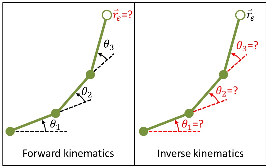
Suppose we have a 2D robot arm consisting of several revolute joints (the solid green circles in the image above) leading up to an end effector (the empty circle in the image above). The end effector might be a gripper or some other sort of robotic manipulator. Each joint is defined by a joint angle, denoted by \(\theta_i\), and the end effector is located someplace in physical space, denoted by the position vector \(\mathbf{r_e}\). Forward kinematics asks, “if we know the joint angles, what are the coordinates \(\mathbf{r_e}\) of the end effector?” On the other hand, inverse kinematics asks, “if we have a desired end effector position \(\mathbf{r_e}\) in mind, what are the joint angles needed to achieve that position?”
Unlike forward kinematics, the answer to the inverse kinematics question is complicated by the fact that it does not always have a single solution.
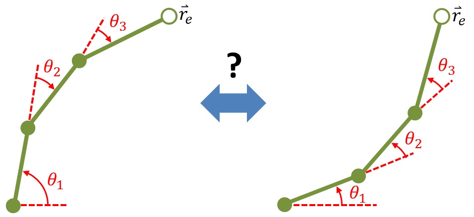
There are usually several orientations, or “poses,” that allow the system to reach the same target end effector position. To further examine this, we must first decide how to describe our robot arm mathematically.
Defining coordinate systems
We’ll be dealing with multiple rotating segments, so it makes sense to define a coordinate system for each joint/segment.
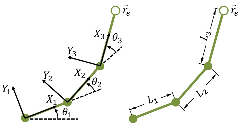
Each joint will serve as the origin for its coordinate system, e.g., \(X_1Y_1\) is the coordinate system for the first joint, where the \(X_1\) axis is coincident with the first link, which has a length \(L_1\). The angle of the first link, i.e., the amount by which the first joint is rotated relative to the global coordinate system, is given by \(\theta_1\). Similarly, the second joint is the origin for the second coordinate system, \(X_2Y_2\), which is rotated by an angle \(\theta_2\) relative to the first coordinate system.
Going from one coordinate system to another can be achieved with transformation matrices. Each joint will have its own transformation matrix. The transformation matrices will allow us to get the coordinates of the end effector in terms of the global coordinate system, which we’ll call the \(X_0Y_0\) system, based on the joint angles and the length of each link.
Even though our robot arm lies in the \(XY\) plane, we’re going to use 3D vectors and 4×4 transformation matrices, not only because we’ll be dealing with cross products, but also because it will help us develop a more general formulation of the inverse kinematics equations. Really, I should be using the notation \(X_iY_iZ_i\) to refer to each coordinate system, since we’ve decided to express the position vectors and transformation matrices in three dimensions, but I’ll stick with \(X_iY_i\) for the sake of keeping things concise. If you aren’t familiar with Euclidean transformations, you can read the previous post.
For the 3-DOF example in this post, with its three revolute joints, we have three transformation matrices:
\[ \left[ ^0 T_1 \right] = \left[ \begin{matrix} \cos{\theta_1} & -\sin{\theta_1} & 0 & x_0 \\ \sin{\theta_1} & \cos{\theta_1} & 0 & y_0 \\ 0 & 0 & 1 & 0 \\ 0 & 0 & 0 & 1 \end{matrix} \right] \]
\[ \left[ ^1 T_2 \right] = \left[ \begin{matrix} \cos{\theta_2} & -\sin{\theta_2} & 0 & L_1 \\ \sin{\theta_2} & \cos{\theta_2} & 0 & 0 \\ 0 & 0 & 1 & 0 \\ 0 & 0 & 0 & 1 \end{matrix} \right] \]
\[ \left[ ^2 T_3 \right] = \left[ \begin{matrix} \cos{\theta_3} & -\sin{\theta_3} & 0 & L_2 \\ \sin{\theta_3} & \cos{\theta_3} & 0 & 0 \\ 0 & 0 & 1 & 0 \\ 0 & 0 & 0 & 1 \end{matrix} \right] \]
where \(\left[ ^0 T_1 \right]\) is the transformation matrix to convert from the \(X_1Y_1\) system to the global \(X_0Y_0\) system (note that \(x_0\) and \(y_0\) are the \(x\) and \(y\) locations of the first joint in the global coordinate system), \(\left[ ^1 T_2 \right]\) is the transformation matrix to convert from the \(X_2Y_2\) system to the \(X_1Y_1\) system, and \(\left[ ^2 T_3 \right]\) is the transformation matrix to convert from the \(X_3Y_3\) system to the \(X_2Y_2\) system.
Finally, the coordinates of the end effector in the \(X_3Y_3\) coordinate system are \(\left\{ \begin{matrix} L_3 & 0 & 0 & 1 \end{matrix} \right\} ^T\).
The coordinates of the end effector can be converted from the \(X_3Y_3\) system to the global \(X_0Y_0\) system by multiplying the transformation matrices with the end effector coordinates in the correct order:
\[ \mathbf{r_e} = \left[ ^0 T_1 \right] \left[ ^1 T_2 \right] \left[ ^2 T_3 \right] \left\{ \begin{matrix} L_3 & 0 & 0 & 1 \end{matrix} \right\} ^T \]
The goal
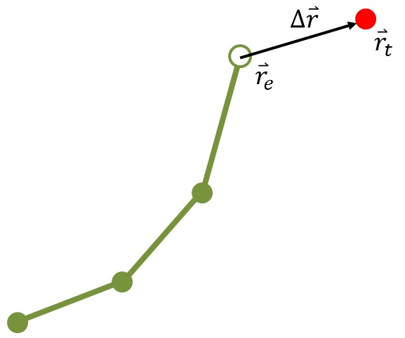
Our aim is to determine how to move the end effector from its current position, \(\mathbf{r_e}\), to a target position, \(\mathbf{r_t}\) (the red dot in the figure above). We’ll call the difference between these \(\mathbf{\Delta r}\), i.e. \(\mathbf{\Delta r} = \mathbf{r_t} - \mathbf{r_e}\). Specifically, we'd like to determine how the joint angles must change for the end effector position to move by \(\mathbf{\Delta r}\). We'll call this change in joint angles \(\mathbf{\Delta}\pmb{\theta}\) (which is a vector containing all the joint angles). This change in joint angles \(\mathbf{\Delta}\pmb{\theta}\) is related to the change in end effector position \(\mathbf{\Delta r}\) by the Jacobian matrix, which we'll cover in the next post.