HOG-based SVM for detecting vehicles in a video (part 6)

This is the sixth and final post in the following series on implementing a HOG-based SVM pipeline to detect objects in a video using OpenCV.

• Part 1: SVMs, HOG features, and feature extraction
• Part 2: Sliding window technique and heatmaps
• Part 3: Feature descriptor code and OpenCV vs scikit-image HOG functions
• Part 4: Training the SVM classifier
• Part 5: Implementing the sliding window search
• Part 6: Heatmaps and object identification

Let’s start, as we’ve been doing, with a video demonstrating the final result:

In the last post, we discussed the sliding window search routine and began to talk about the detector itself, implemented via the Detector class. The code and additional information about the project are available on Github. I won’t touch on every remaining line of code, as that would be excessive and counterproductive—for a full understanding of what the Detector is doing to achieve the result in the video above, you can check out the source code, the project README, and the program usage INSTRUCTIONS. I will, however, attempt to touch on high-level implementation details and the relevant parts of the source code.

Building a heatmap to sum overlapping detections

If our SVM has been trained properly, it should identify vehicles in a video with relatively few false positives. Still, there will likely be a handful of false positives. Moreover, there’s no guarantee that each vehicle will only be detected once, in a single window, during the sliding window search. Since our windows overlap, there’s a not insignificant chance that the same object will be detected in multiple windows. If we run the detector and display only the raw sliding window detections without any additional processing, this is exactly how it turns out. In the following video, each green bounding box represents a window from the sliding window search that the SVM classified as “positive,” i.e., containing a vehicle. Note that the sliding window search is performed at every frame of the video.

These detections are produced by Detect.classify(), which converts an image to the appropriate color space, builds a list of feature vectors—one for each window in the sliding window—then scales all the feature vectors before running them through the classifier.

77
78
79
80
81
82
83
84
85
86
87
88
89
90
91
92
93
94
95
96
97
98
99

def classify(self, image):

    """
    Classify windows of an image as "positive" (containing the desired
    object) or "negative". Return a list of positively classified windows.
    """

    if self.cv_color_const > -1:
        image = cv2.cvtColor(image, self.cv_color_const)

    if len(image.shape) > 2:
        image = image[:, :, self.channels]
    else:
        image = image[:, :, np.newaxis]

    feature_vectors = [self.descriptor.getFeatureVector(
            image[y_upper:y_lower, x_upper:x_lower, :])
        for (x_upper, y_upper, x_lower, y_lower) in self.windows]

    # Scale feature vectors, predict, and return predictions.
    feature_vectors = self.scaler.transform(feature_vectors)
    predictions = self.classifier.predict(feature_vectors)
    return [self.windows[ind] for ind in np.argwhere(predictions == 1)[:,0]]

The issue of multiple detections is a good problem to have, since it means the SVM classifier is working. The method I’ve chosen to combine these repeated detections is a heatmap, which can be found in the Detector class method Detector.detectVideo():

167
168
169
170
171
172
173
174
175

current_heatmap[:] = 0
summed_heatmap[:] = 0
for (x_upper, y_upper, x_lower, y_lower) in self.classify(frame):
    current_heatmap[y_upper:y_lower, x_upper:x_lower] += 10

last_N_frames.append(current_heatmap)
for i, heatmap in enumerate(last_N_frames):
    cv2.add(summed_heatmap, (weights[i] * heatmap).astype(np.uint8),
        dst=summed_heatmap)

current_heatmap is a 2D numpy array of the same width and height as the source video. At each iteration of the loop, i.e., for each frame, we set all its elements equal to 0 on line 167. This is why I’ve named it current_heatmap —because it’s the heatmap for the current frame, which we recompute at each frame. On lines 169-170, we iterate through all the positively classified windows for the current frame and increment the pixels in the heatmap corresponding to the pixels contained within the window. I’ve arbitrarily chosen an increment of +10. Every time a pixel is part of a positively classified window, its value will be incremented in the heatmap by +10. Therefore, pixels in regions with a large number of overlapping detections will end up with relatively large values in the heatmap.

To smooth the heatmap, I also opted to store the heatmaps from the last N frames in a deque (line 172) and sum all the frames in the deque. The number of frames N can be set by the user. A deque, or double-ended queue, is a data structure whose length, in Python, can be fixed. When the deque reaches maximum capacity, appending a new element to the back of the deque automatically pops the element at the front. In this case, the element at the front is the oldest heatmap. While summing the heatmaps in the deque to produce what I’ve called the summed_heatmap on lines 173-175, I’ve also applied a weighting to the heatmaps; older frames are given less weight than more recent frames.

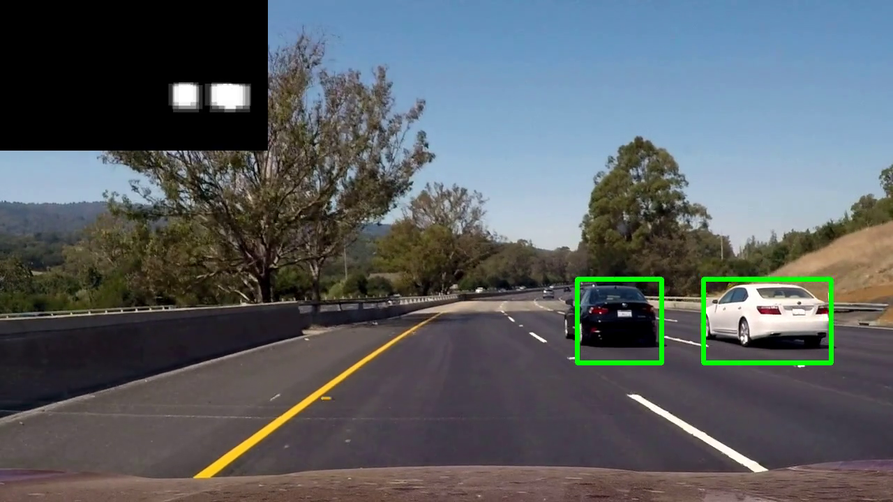
Although the final result displays a small, grayscale heatmap in the upper left-hand corner of the video, it might help to visualize the heatmap by superimposing it on the video at full scale. The following video does exactly that using the color red:

To reduce the number of false positives, we keep only those pixels of the heatmap that exceed a certain threshold and set the rest to 0 on line 189:

189

summed_heatmap[summed_heatmap <= threshold] = 0

Having constructed a heatmap of detections that takes into account the last several frames, we can now proceed with separating the remaining “blobs” on the heatmap into distinct objects.

Identifying and boxing distinct objects

Next, we apply a connected component algorithm to determine which pixels in the heatmap belong to the same object. Luckily, scipy offers this functionality via the scipy.ndimage.measurements.label() method, which we employ on line 192:

192

num_objects = label(summed_heatmap, output=heatmap_labels)

This function returns an array, which I’ve called heatmap_labels, of the same size as summed_heatmap, where elements corresponding to pixels that are part of the first object are set to “1”, elements corresponding to pixels that are part of the second object are set to “2”, and so on for as many objects as were found (which, of course, might be zero). If we were to stop here and display the results of labeling the blobs in the heatmap, it would look something like this:

Moving on, we iterate through each object label (1, 2, 3, etc.) on lines 195-204, at each iteration isolating only the pixels in heatmap_labels corresponding to the current object label. By obtaining the minimum and maximum x and y coordinates, respectively, of each object, we can draw the largest possible bounding box around it.

195
196
197
198
199
200
201
202
203
204

for obj in range(1, num_objects + 1):
    (Y_coords, X_coords) = np.nonzero(heatmap_labels == obj)
    x_upper, y_upper = min(X_coords), min(Y_coords)
    x_lower, y_lower = max(X_coords), max(Y_coords)

    # Only draw box if object is larger than min bbox size.
    if (x_lower - x_upper > min_bbox[0]
            and y_lower - y_upper > min_bbox[1]):
        cv2.rectangle(frame, (x_upper, y_upper), (x_lower, y_lower),
            (0, 255, 0), 6)

This, ultimately, provides the final result—the video at the beginning of this post.

Final thoughts

You can read about the results and conclusions, as well as the parameters I used, in more detail in the README on Github. However, I will say that this project was more a learning experience than anything else, at least for me, though one that demonstrated the utility of SVMs and HOG features as methods for object detection. At about 3 frames of video processed per second on my hardware, this particular implementation ended up being too slow for any real-time application. And, though I’m sure its performance could be improved by incorporating parallelism in the form of multithreading and multiprocessing, or by rewriting the code to use Cython (topics I may cover in a future post), or by simply rewriting the pipeline in C++, I would argue that these tasks would be exercises with more educational value than practical value. After all, there’s a reason HOG and SVM have been supplanted by deep learning and convolutional neural networks, which tend to achieve both high accuracy and extremely fast speeds.

Regardless, don’t discount the utility of SVM as a machine learning technique that can be applied to a wide variety of challenges both within and outside the realm of computer vision.