
This post is part of a series on developing an SVM classifier to find vehicles in a video:
- Part 1: SVMs, HOG features, and feature extraction
- Part 2: Sliding window technique and heatmaps
- Part 3: Feature descriptor code and OpenCV vs scikit-image HOG functions
- Part 4: Training the SVM classifier
- Part 5: Implementing the sliding window search
- Part 6: Heatmaps and object identification
The code is also available on Github. In this post, we’ll examine the portion of the vehicle detection pipeline after the SVM has been trained. Once again, here’s the final result:
The sliding window technique
The goal of our vehicle detection SVM is to classify an image as “vehicle” or “non-vehicle”. For this project, I trained the SVM on 64×64 patches that either contained a vehicle or didn’t contain a vehicle. A blown-up example of each (as well as its HOG visualization) is presented again below:
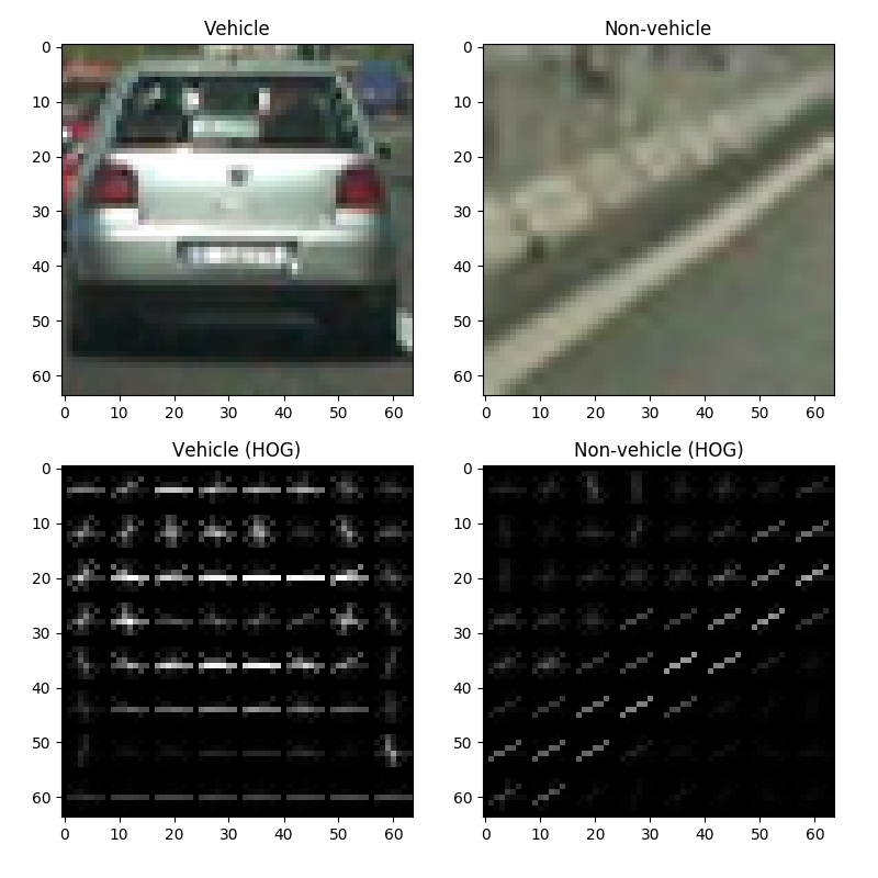
These images were obtained from the Udacity dataset, which contained 8799 64×64 images of vehicles and 8971 64×64 images of non-vehicles, all cropped to the correct size. These images are actually subsets of the GTI and KITTI vehicle datasets, if you’d like to check those out.
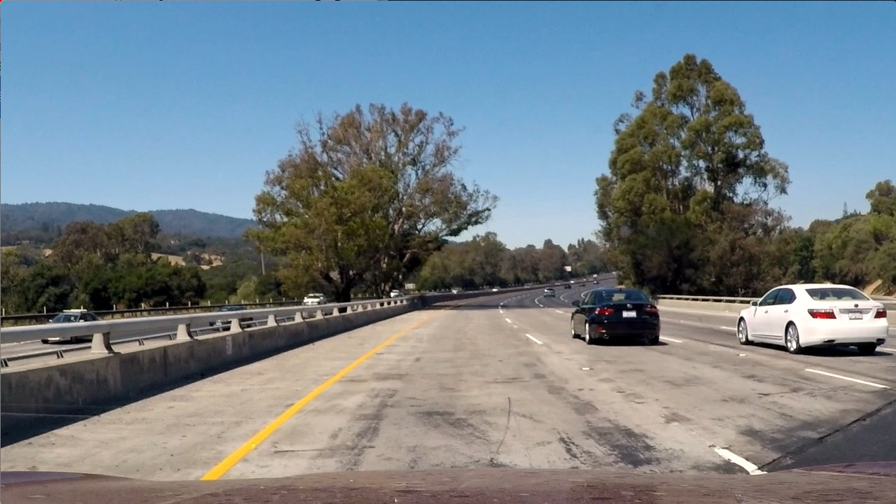
However, actual frames of a video won’t be nicely cropped 64×64
images. Instead, they’ll look something like this:
To find vehicles in a full image, we utilize a sliding window. Traditionally, this involves selecting a window of a relatively small size, like 64×64 or 100×100, etc., and “sliding” it across the image in steps until the entirety of the image has been covered. Each window is fed to the SVM, which classifies that particular window as “vehicle” or “non-vehicle”. This is repeated at several scales of the image by scaling the image down. Sampling the image at different sizes helps ensure that instances of the object both large and small will be found. For example, a vehicle that’s nearby will appear larger than one that’s farther away, so downscaling improves the odds that both will be detected. This repeated downscaling of the image is referred to as an “image pyramid.” Adrian Rosebrock has a good set of posts on using sliding windows and image pyramids for object detection over at pyimagesearch.
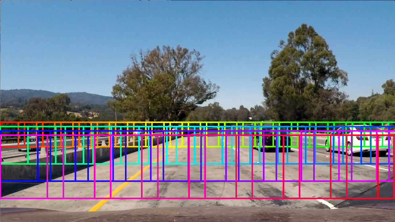
In my implementation, I originally utilized a sliding window of fixed size sampling different scales of the image via an image pyramid, but found it to produce many false positives. As an alternative, I tried a sliding window of variable size with a relatively small initial size that increased in size with each step toward the bottom of the image, the rationale being that vehicles near the bottom of the image are physically closer to the camera and appear larger (and vice versa). Furthermore, I only scanned the portion of the image below the horizon, since there shouldn’t be any vehicles above the horizon. This seemed to improve the results significantly. The following short clip demonstrates the technique:
Observe that there’s considerable overlap between windows:
This means that the same vehicle will probably be detected multiple times in adjacent windows, which ends up looking like this:
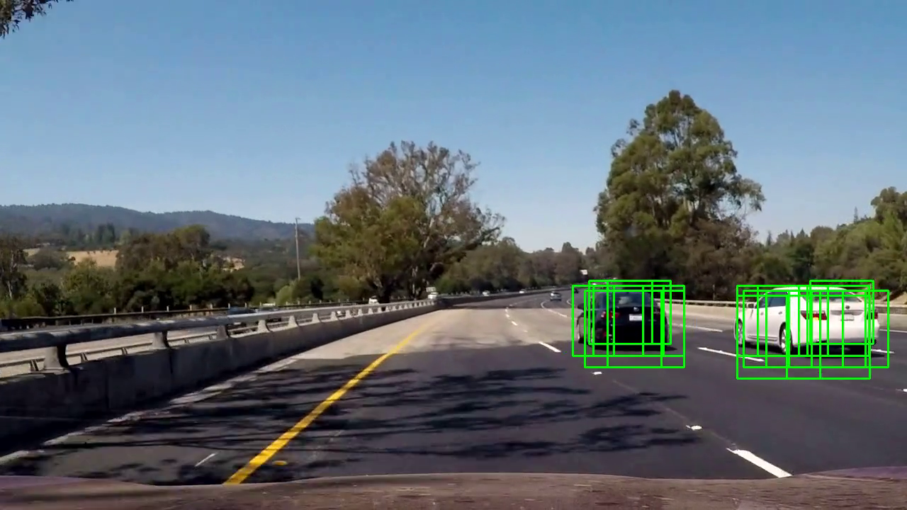
The full video, with all detections drawn at every frame:
However, our goal is to find (and draw a box around) individual vehicles. To do this, we must reduce multiple overlapping detections into a single detection, which we’ll explore in the next section.
IMPORTANT NOTE ON WINDOW SIZES: Recall that the features extracted from each window will be fed to and classified by the SVM (as “positive” / “vehicle” or “negative” / “non-vehicle”). If the SVM was trained on 64×64 images, the features extracted from each window must also come from a 64×64 image. If the window is a different size, then each window should be resized to 64×64 before feature extraction—otherwise, the results will be meaningless.
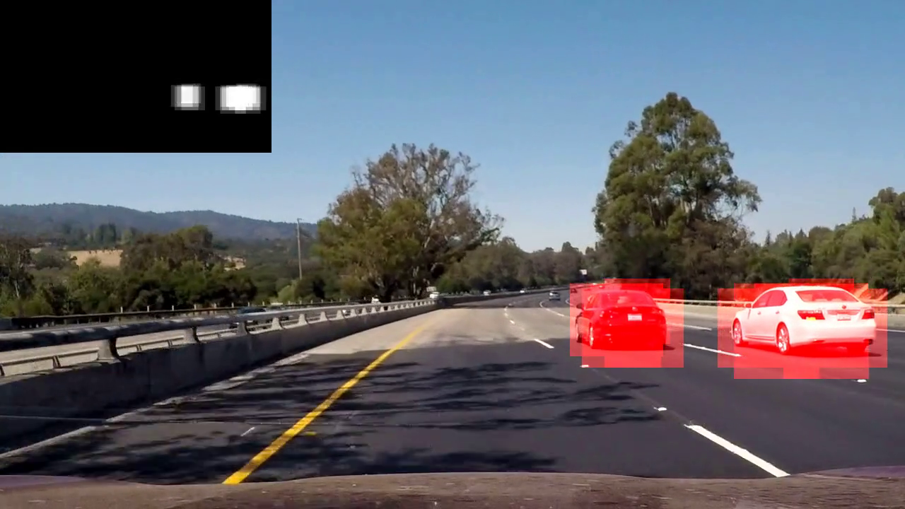
Heatmap for combining repeated detections
Several methods exist for reducing repeated detections into a single detection. One approach is to build a heatmap in which each detection contributes some positive value to the region of the image it covers. Regions of the image with many overlapping detections will provide a greater number of contributions to that region of the heatmap, seen in the image below (the full-scale heatmap superimposed on the raw image uses shades of red instead of grayscale like the small-scale inset heatmap in the corner):
To reduce false positives, we can use the weighted sum and/or average of the heatmaps of the last N frames of the video, giving a higher weight to more recent frames and a lower weight to older frames, then consider only areas of the summed heatmap with values above some threshold. This way, regions with consistent and sustained detections are more likely to be correctly identified as vehicles, while areas with fleeting detections that only last a couple frames (which are likely false positives) are more likely to be ignored. Here’s the complete video with the full-scale superimposed heatmap:
Labeling and boxing distinct objects
Having combined multiple detections into “blobs” on the heatmap, we can now apply a connected-component algorithm to determine how many distinct objects (blobs) are present, as well as which pixels belong to which object:
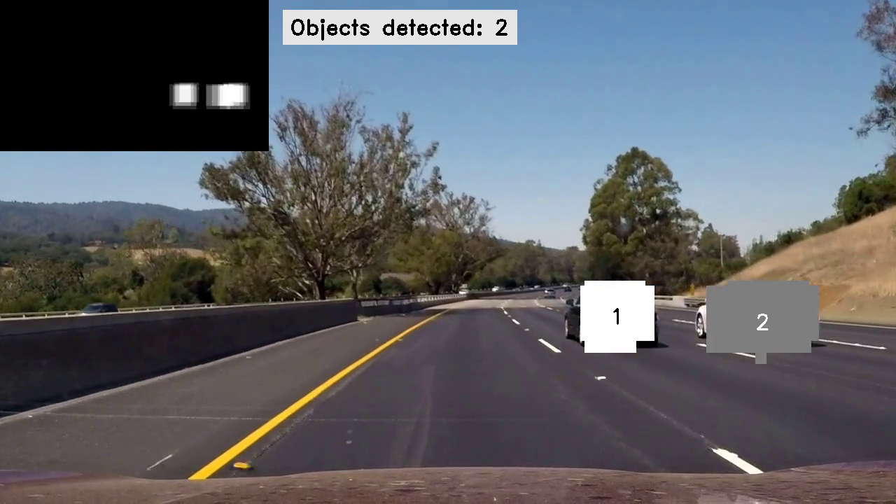
And, of course, the full video with each object labeled with a unique identifier (number):
This video demonstrates an important fact: objects are numbered arbitrarily and sometimes change numbers between frames. In other words, this algorithm detects objects but does not track them.
The final step, after finding each object, is to draw the largest possible bounding box around each object, ignoring objects that are too small and likely to be false positives.
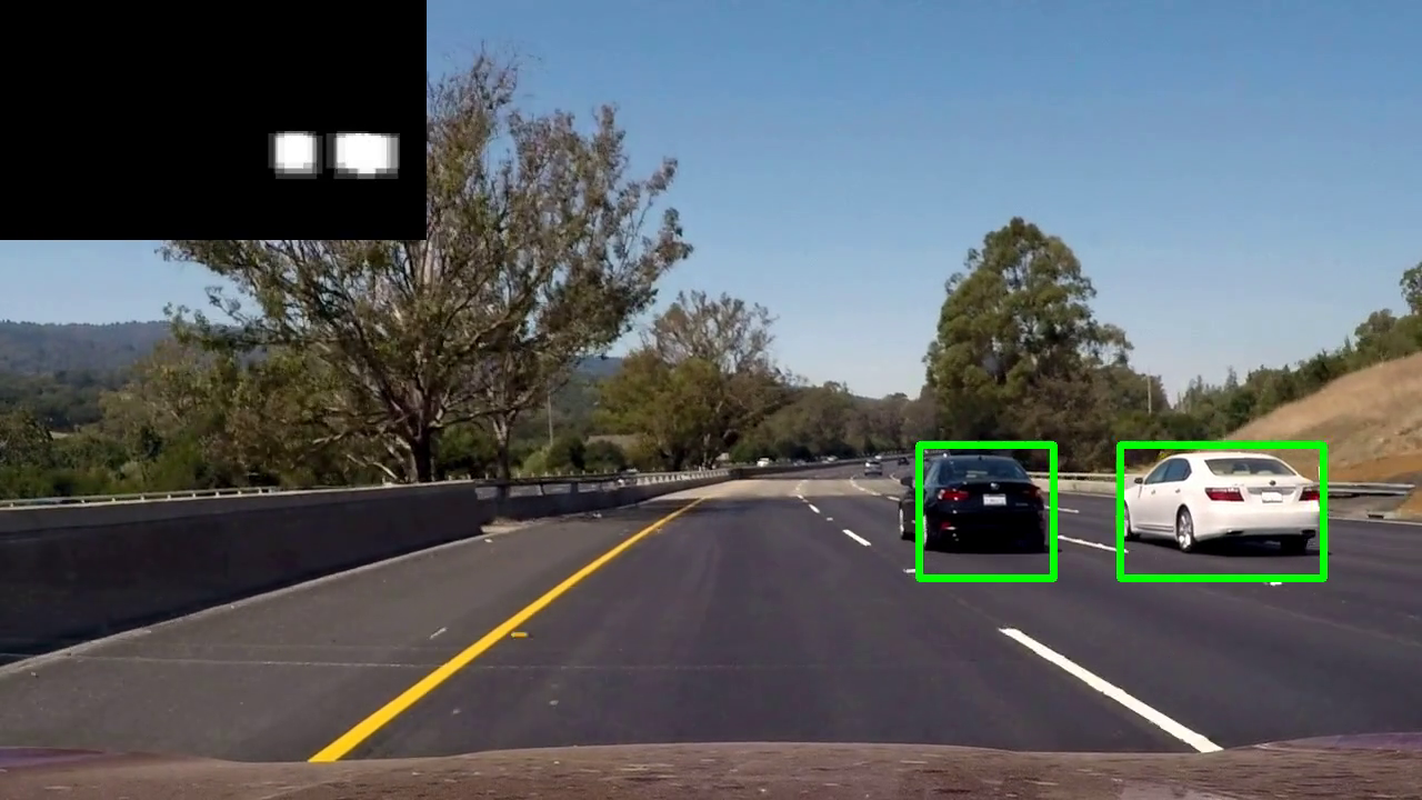
In the next post, we’ll delve into finer implementation details and specifics by examining the code.