
Computer vision and machine learning often attempt to replicate tasks that most of us take for granted. As you might guess from the title of this post, identifying other vehicles on the road is one of those tasks—one that anyone who’s driven or sat in a car is familiar with. How can we teach a computer to do the same? In this series of posts, we’ll discuss a method involving a HOG-based SVM for finding and tracking vehicles in a video. Don’t worry if you’re not familiar with these terms—we’ll go through the relevant topics.
- Part 1: SVMs, HOG features, and feature extraction
- Part 2: Sliding window technique and heatmaps
- Part 3: Feature descriptor code and OpenCV vs scikit-image HOG functions
- Part 4: Training the SVM classifier
- Part 5: Implementing the sliding window search
- Part 6: Heatmaps and object identification
First, let’s see what the end result looks like:
In the video above, you can see green bounding boxes drawn around cars. The inset in the upper left corner displays a “heatmap”. The heatmap is simply a scaled-down version of the actual video, in which white signifies areas of high prediction density (i.e., areas where the detector strongly predicts there’s a car) and black signifies areas of low prediction density (areas where the detector doesn’t predict there’s a car). The final result isn’t perfect—the bounding boxes are a little shaky and detector occasionally picks up false positives—but it works, for the most part. If you’d like, you can check out the project and source code on Github.
Let’s dive into the detection pipeline. In this post, we’ll learn about SVMs and HOG features, as well as color histogram features and spatial features.
What is an SVM?
SVM stands for “support vector machine”. An SVM is what’s known as a “classifier,” meaning it classifies something as belonging (or not belonging) to a certain group, also called a “class”. For example, you might develop an SVM that determines whether something is a car or whether it’s a truck based on its features. A “feature” is anything that describes the input. We might choose our features to be the length of a vehicle and the weight of a vehicle. To prepare our SVM, we must first train it on a labeled dataset, i.e., a set of training samples for which the class of each sample— “car” or “truck”—is already known. Based on this training data, the SVM figures out what distinguishes a car from a truck, like so:
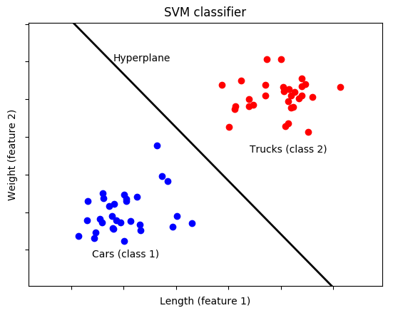
In this simple example, training samples corresponding to cars are represented by blue dots and training samples corresponding to trucks are represented by red dots. Each axis (dimension) represents a feature—in this case, length and weight. Observe how the points for the two classes are positioned along the two dimensions, with cars tending to be shorter and lighter than trucks. The SVM computes the optimal “hyperplane” that separates the two classes based on their features. In this case, we only have two dimensions (features), so the hyperplane is just a line.
Our hypothetical SVM has, at this point, been trained. Now, we can feed it features from a new, unlabeled sample and it will, based on the length and weight of the unknown vehicle, classify it as a “car” if it falls on one side of the hyperplane and a “truck” if it falls on the other side.
Granted, this is a gross oversimplification, but it does demonstrate an important point: an SVM doesn’t care what the input features are. In other words, its utility is not limited to images. An SVM can be trained on anything, so long as we can extract features from the input data. This begs the question: what features can we extract from an image to determine whether it contains (or doesn’t contain) a certain object? For vehicle detection using an SVM, a popular answer turns out to be HOG features.
What are HOG features?
“HOG” stands for “histogram of oriented gradients”. I’ll only go into HOG features briefly here, as there are a lot of great resources on the topic available elsewhere online. Personally, I found Satya Mallick’s post over at Learn OpenCV to provide a clear and concise explanation. If you’re looking for a more formal, detailed treatment of HOG, I would highly recommend reading the original paper on HOG features by Dalal and Triggs, titled “Histograms of Oriented Gradients for Human Detection”.
The basic idea behind HOG is to use edges to describe the content of an image. For example, say we wanted to develop an SVM to find people in an image. Picture the outline (“edges”) of a person compared to, say, the outline of a tree or a car. They’re pretty different, right? HOG seeks to quantify these differences in edge shapes to differentiate objects from one another. Edges can be described in terms of the gradient (the “G” in “HOG”) of each pixel in an image. The Sobel operator is one method that can be used to compute the gradient in both the x and y directions for each pixel. If you’re not familiar with gradients or the Sobel operator, check out this previous post. Essentially, the magnitude and direction of the gradient are computed for each pixel as follows:
\[G = \sqrt{G_x^2 + G_y^2}\]
\[\theta = \arctan{\frac{G_y}{G_x}}\]
where \(G\) is the magnitude of the gradient, \(G_x\) is the gradient in the x direction, \(G_y\) is the gradient in the y direction, and \(\theta\) is the direction of the gradient.
Next, the image is divided into groups of pixels called “cells.” For instance, we might choose a cell size of 8×8 (8 pixels by 8 pixels), giving us a total of 64 pixels per cell. Recall that each pixel has two associated values: gradient magnitude and gradient direction, where the direction is also known as its “orientation,” hence the “oriented” in “histogram of oriented gradients.” Also recall that the orientation is an angle between 0°-360° or, if we don’t care about the sign of the angle, an angle between 0°–180°. The next step is to create a histogram of each cell by dividing the range of orientations into bins. For example, we might choose 9 bins which, for unsigned gradients, would give us bins with edges at 0°, 20°, 40°, and so on up to 160° (since 0° and 180° are identical in the case of unsigned gradients). Each of the 64 pixels in a cell votes toward these bins based on its magnitude and orientation. If you’re keeping score, that gives us 9 values per cell.
We can attempt to visualize the HOG features of an image by plotting the bins for each cell in an image, which looks like this:
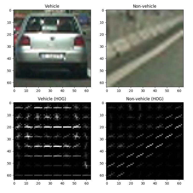
In the figure above, we have 64×64 images of a vehicle (the back of a car) and a non-vehicle (the side of a highway), blown up to help us see what’s going on. Each cell contains a histogram depicted by crisscrossing lines representing bins—the horizontal line for each cell represents the 0° bin, the least slanted diagonal line represents the 20° bin, and so on. The brightness of each bin (line) represents the magnitude of that bin, so a bright white horizontal line signifies that the gradient for that cell is primarily horizontal. Ultimately, the images help us visualize the difference between a vehicle and non-vehicle in terms of their gradients—or, more specifically, in terms of the histograms of their gradients.
For a 64×64 image with a cell size of 8×8, as in the images above, there are 64 cells, each with 9 values. However, HOG features are sensitive to local lighting and noise, so we go a step further and group cells into blocks, then normalize each block based on the magnitude of the all the values in that block. If we choose a block size of 2×2 (2 cells by 2 cells), that works out to 4 cells per block times 9 values per cell for a total of 36 values per block. If we shift the block one cell at a time (each time normalizing the 36 values relative to the magnitude of those 36 values) both horizontally and vertically to cover every possible 2×2 combination of cells, we end up with 36 values per block times 49 blocks (7 horizontal positions times 7 vertical positions) for a grand total of 36 * 49 = 1764 values for a 64×64 image.
These 1764 values are our HOG features. While we can’t visualize a 1764-dimensional feature space, it’s the exact same idea as our earlier car/truck example, in which we only had two dimensions (features), length and weight, and could easily visualize separating the two classes with a line. If we had three features (three dimensions), we could visualize the two classes being separated by a plane. In any arbitrary number of dimensions, the two classes are separated by the aforementioned hyperplane.
Additional features
In addition to HOG features, we can add other features to our “feature vector” (which, at present, contains 1764 values from the HOG feature descriptor), if we so desire. In my implementation, I’ve included the color histogram of an image, since the color profile of vehicles will, generally speaking, be different from the color profile of the surrounding environment (gray road, green trees, etc.). This simply entails dividing the values in color depth of an image into bins, computing the histogram for each color channel, and appending the resulting values to our feature vector. For a primer on computing histograms for the channels of an image, see this previous post.
I’ve also included spatial features—in other words, the raw values of the channels for each pixel. This helps capture spatial relationships between points in an image. Of course, in a 64×64 image, there are 4096 pixels. For a three-channel image, that would be an additional 4096 * 3 = 12288 features. To avoid making our feature vector too large, we can resize the image to a smaller size, like 16×16 (256 pixels, or 768 features for three channels), before adding these spatial features to the feature vector.