
UPDATE (2019-05-05): The code is now available on
Github! It can be installed as a package,
and the file example.py in the root directory can be run for demonstration
by executing the following commands in a terminal:
$ git clone https://github.com/nrsyed/half-car.git
$ cd half-car
$ pip install -e .
$ python example.py
The original post follows below.
“Vehicle dynamics” is a delightfully broad term that, in equally broad terms, refers to how vehicles move. As the title of this post suggests, we’ll be looking at cars, although the techniques we’ll use can be applied to any wheeled vehicle with suspension. So, what, exactly, is a “half-car suspension model”? It can be animated like this:
In the video above, we get an idea of the pitch and bounce dynamics of a car, when viewed from the side, in a variety of conditions. The little triangles in some of the clips are “roadside markers” placed at 10 meter intervals to help visually gauge the speed of the car. Note that, even though only springs are displayed to represent the suspension in the video, both the front/rear suspension and the front/rear wheels are modeled as springs and dampers, as we’ll see below.
The rest of this post will look at the underlying principles behind this half-car model and briefly discuss the numerical approach employed to solve the dynamics of the system.
Basic setup
A car is a vehicle with a chassis connected to four wheels (usually). These four wheels, in turn, are in contact with the road. The chassis isn’t directly attached to the wheels—rather, it is connected to them by the suspension, which generally consists of coil springs and shock absorbers (dampers). In other words, the interface between the chassis and each wheel is a spring and damper. In the automotive world, the chassis is called the sprung mass, since it is the portion of the vehicle held up by springs. In contrast, each wheel is referred to as an unsprung mass. Of course, the term “unsprung mass” is ever-so-slightly misleading, because we can also model the tire as a spring and damper. An inflated rubber tire is essentially a very stiff spring.
If we took one corner of the car, i.e., one tire and a quarter of the chassis, it would look like this:
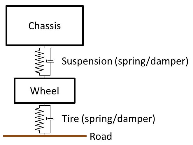
This is called a quarter-car suspension model. It’s a one-dimensional system comprising a sprung mass (one quarter of the chassis) and an unsprung mass (the wheel). These form a 2-DOF system characterized by a pair of differential equations, which are obtained by summing forces in the vertical direction for the chassis and summing forces in the vertical direction for the wheel. Similarly, a half-car suspension model considers half the car. Sometimes, a half-car model considers the front half or rear half of the car (and their associated roll dynamics) but, usually, “half-car model” refers to the left/right halves and their pitch and bounce dynamics:
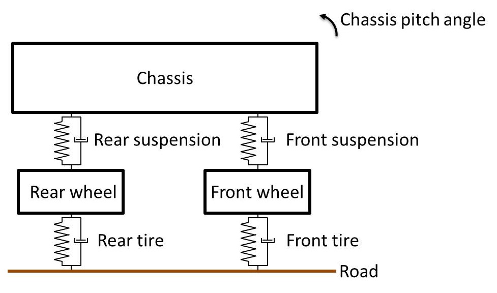
This is a 4-DOF system described by the vertical displacement of the front wheel, the vertical displacement of the rear wheel, the vertical displacement of the chassis (i.e., the “bounce”), and the rotation angle of the chassis (i.e., the “pitch”). We will need four equations to describe it. Before delving into that, let’s change the appearance of our car to look more like an actual car. This isn’t necessary, of course, but it might make the problem easier to visualize and, more importantly, it looks cooler. For no particular reason, let’s choose a 2010 Honda Accord Coupe:
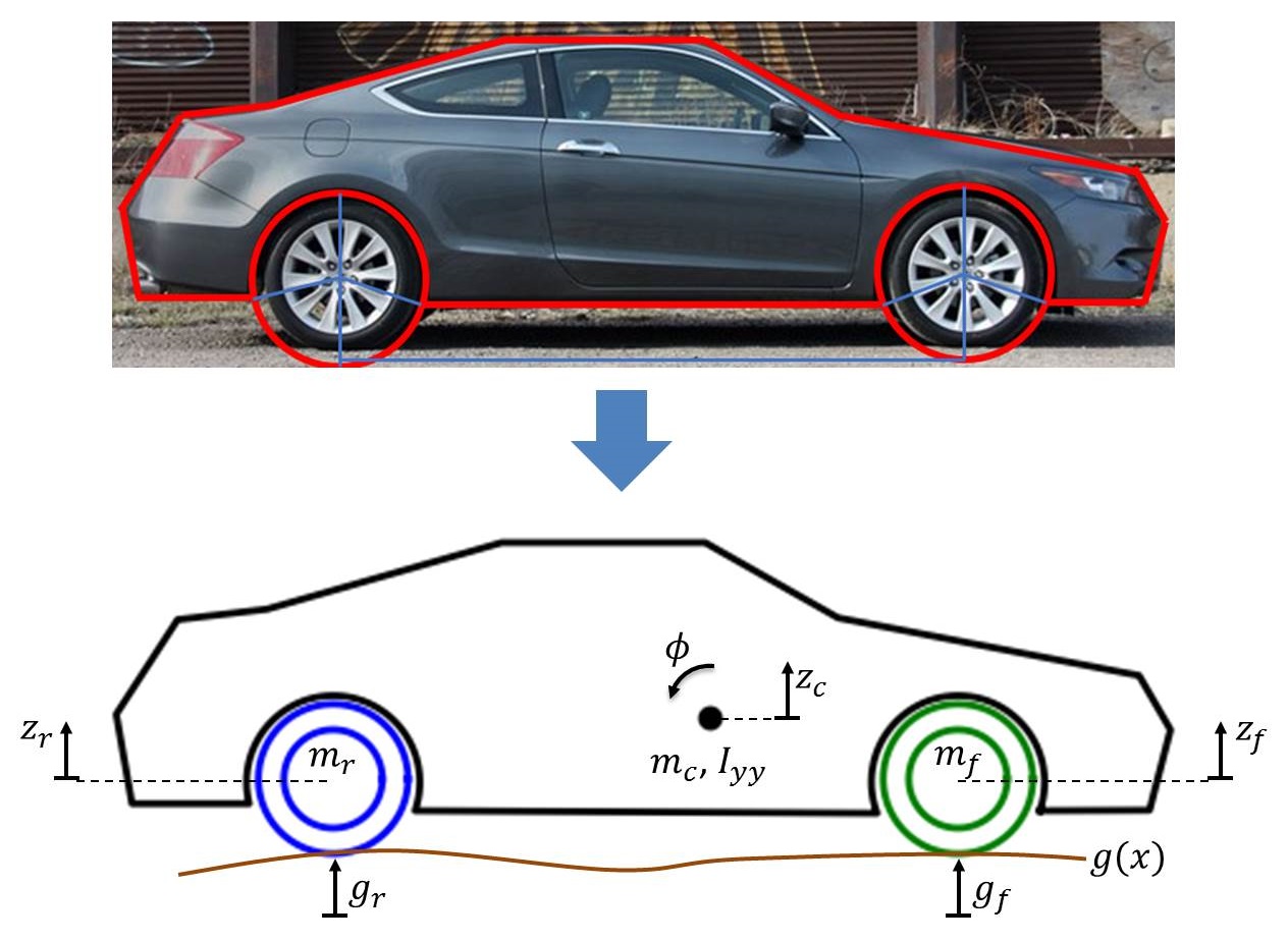
The figure above defines several coordinates and variables. \(z_c\) is the vertical displacement of the chassis center of mass (COM) from its initial position, \(\phi\) is the pitch angle of the chassis, \(z_f\) is the vertical displacement of the front wheel COM from its initial position, and \(z_r\) is the vertical displacement of the rear wheel COM from its initial position. \(g(x)\) is the forcing function, i.e., the road, and represents the vertical displacement of the road at any given horizontal coordinate \(x\) along the road. \(g_f\) and \(g_r\) are the value of this function at the front and rear wheel points of contact, respectively. \(m_c, m_f, m_r\) are the masses of the chassis, front wheel, and rear wheel, respectively, and \(I_{yy}\) is the mass moment of inertia of the chassis about the pitch axis (y axis).
Forces and equations of motion
First, let’s look at the forces acting on the system as a whole:
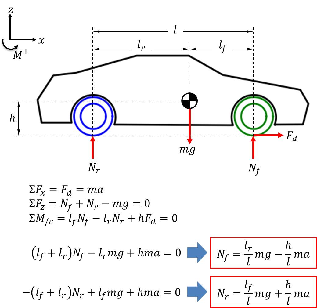
\(l_f\) is the distance from the chassis COM and the point where the front suspension attaches to the chassis. This is where the forces due to the front suspension spring and damper will act on the chassis. Similarly, \(l_r\) is the distance to the rear suspension attachment point. \(F_d\) is the drive force responsible for accelerating the car. Observe that there’s only one drive force and that it’s acting at the front wheel, since this is a front-wheel-drive car. To keep things simple (and because the effect is the same, dynamically), we’ll consider a negative drive force to be a braking force, even though the car has both front and rear brakes. The drive (or braking) force is related to the car’s acceleration by \(F_d = ma\), where \(m\) is the total mass of the car (\(m = m_c + m_f + m_r\)) and \(a\) is the horizontal acceleration of the car. Note that the system’s overall COM won’t be at exactly the same location as the chassis COM, since it also accounts for the COM of each wheel, but because the mass of the chassis is significantly larger than the mass of the wheels, it will be relatively close. For simplicity, we’ll proceed with the assumption that the chassis COM and the system COM are identical. The figure above and the equations therein show us that the normal force acting on each wheel consists of a static component and a dynamic component. For the front wheel, the static component is \(\frac{l_r}{l}\ mg\) and the dynamic component is \(-\frac{h}{l}\ ma\). For the rear wheel, the static component is \(\frac{l_f}{l}\ mg\) and the dynamic component is \(\frac{h}{l}\ ma\). Here, the wheelbase \(l\) is defined as \(l = l_f + l_r\) and \(g\) refers to gravity, not the road function from above. This means that the normal forces acting on the wheels change proportionally with acceleration. This is why the back of a car dips (“squats”) when it accelerates and why the front of a car dips (“dives”) when it brakes.
This also brings up another important point: the static component of the normal force depends only upon the mass of the car and the positions of the wheels relative to the overall COM. It doesn’t change regardless of acceleration. Recall how, several paragraphs above, all the coordinates were defined as displacements from an initial position; for convenience, we can define that initial position to be when the car is at rest on flat ground. Then, studying the dynamics of this multibody system is just a matter of examining what happens when the components of the car or the forces acting on the car change. In other words, we can assume all static forces are taken into account by the initial position. For example, we can ignore the weight \(m_c g\) of the chassis because the springs in the suspension are already sufficiently compressed (pre-loaded) to offset it in the initial position. Similarly, we can ignore the static parts of the normal forces and take into account only the dynamic (changing) parts, which I’ll call \(\Delta N_f\) and \(\Delta N_r\). Keeping this in mind, we can now continue by examining each rigid body and writing its equation(s) of motion, starting with the chassis:
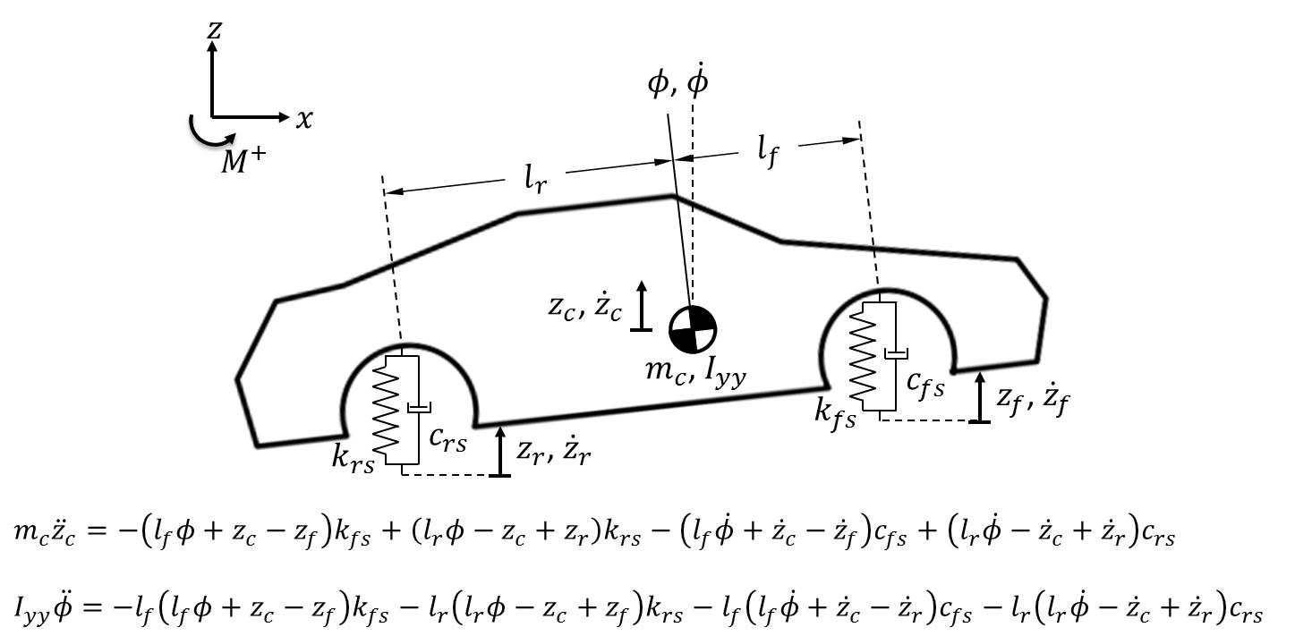
\(k_{fs}\) and \(k_{rs}\) are the spring rates of the front suspension and rear suspension, respectively. \(c_{fs}\) and \(c_{rs}\) are the damping constants of the front and rear suspension. There are two equations of motion for the chassis, one for its vertical translation (bounce) and the other for its rotation (pitch). Although the pitch angle in the figure above is exaggerated for effect, it’s assumed that the chassis will pitch through a relatively small range of angles. Therefore, we utilize the small angle approximation \(sin\theta \approx \theta\) in the moment equation. Observe that we utilize both the position and velocity of each coordinate—position for the spring forces and velocity for the damper forces. Also note that we assume the suspension remains vertical, regardless of the chassis pitch angle; this goes hand-in-hand with the small angle approximation. For small angular displacements, these assumptions are valid approximations.
Next, we write the equations of motion for the vertical displacement of each wheel:
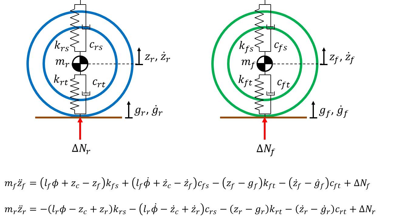
\(k_{ft}\) and \(k_{rt}\) are the spring rates of the front and rear tires, respectively. Similarly, \(c_{ft}\) and \(c_{rt}\) are the damping constants of the front and rear tires. Notice that the forces of the suspension acting on the wheels are equal and opposite to the forces of the suspension acting on the chassis.
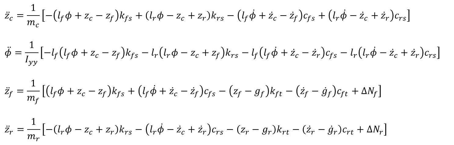
Writing all four equations together and solving for the accelerations by dividing through the masses and mass moment of inertia:
Finally, we can rewrite this system of equations in matrix form. Multiplying the terms through (and separating them into corresponding matrices/vectors) is left as an exercise to you, the reader, but the end result looks like this:
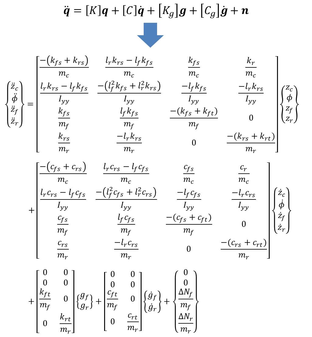
If you’re not used to dealing with matrices, this might seem intimidating at first, but all it does is reorganize our four equations of motion into several distinct pieces. \(\pmb{\ddot{q}}\) is a 4×1 vector containing the acceleration of the coordinates \(\{z_c, \phi, z_f, z_r\}^T\), which I’ve denoted as a vector \(\mathbf{q}\) (from which it follows that \(\mathbf{\dot{q}}\) is a vector containing the velocity of each coordinate). \([K]\) is the stiffness matrix that consolidates the spring constants and \([C]\) is the damping matrix that consolidates the damping constants. \(\mathbf{g}\) and \(\mathbf{\dot{g}}\) are vectors containing the displacement and velocity, respectively, of the road at the front and rear points of contact with the wheels. To go along with these are \([K_g]\) and \([C_g]\), which relate the road profile (and its rate of change) to forces exerted on the wheels. Finally, the vector \(\mathbf{n}\) is a normal force vector containing the dynamic parts of the normal force at the front and rear wheels. Splitting all of these up into matrices and vectors makes it relatively easy to solve the dynamics of the system numerically, since the matrices contain properties of the system that do not change, whereas the vectors can be updated at each iteration.
Numerical solution via the Euler method
There exist many robust and stable numerical methods for solving a system of differential equations like this one. The Euler method is not one of them. Why did I choose it for this post, then? Because it’s simple, relatively speaking, and requires little more explanation than we’ve already been through. Instead of going into detail about the Euler method (which can essentially be thought of as a first order Runge-Kutta method, if you’re familiar with RK methods), I’ll just show you how it works, in the context of this particular problem, with four fairly straightforward equations:
\[\mathbf{q}_0 = \mathbf{q}(0)\]
\[\mathbf{\dot{q}}_0 = \mathbf{\dot{q}}(0)\]
\[\mathbf{q}_{i+1} = \mathbf{q}_i + \mathbf{\dot{q}}_i \Delta t\]
\[\mathbf{\dot{q}}_{i+1} = \mathbf{\dot{q}}_i + \mathbf{\ddot{q}}_i \Delta t\]
The first two equations just set the initial positions and initial velocities to whatever we choose. The third equation computes the positions at the next iteration based on the current positions and velocities. The fourth equation computes the velocities at the next iteration based on the current velocities and accelerations. We select a time step \(\Delta t\) for our simulation, which is applied at every iteration. The smaller the time step, the more accurate the simulation. We apply these last two equations repeatedly until the algorithm reaches a selected end condition, or indefinitely, if we wish.
That, in a nutshell, is a simple numerical approach to solving half-car dynamics. There are many other methods, both numerical (like the aforementioned Runge-Kutta methods) and analytical (like developing and solving the transfer function for the system). While numerical approaches have disadvantages, like the potential for instabilities and error, they also have advantages, like the ability to easily handle nonlinear inputs (e.g., random road profiles). We may explore some of these other approaches in future posts. Furthermore, the next step up from a half-car model is a full-car model. As you might guess, a full-car model is a three-dimensional model with considerably more degrees of freedom, which takes into account the roll, pitch, and yaw of the vehicle, as well as the vertical displacements of four wheels. We may tackle this in a future post, as well.