DC motors, which have been around in one form or another since the 19th century, are common in many applications and industries. You can find them in consumer products and medical devices, and hobbyists frequently use them in RC cars and quadcopters. There are several types of DC motors, the most common being permanent magnet DC (PMDC) “brushed” or “brushless” motors. These are most likely what you’ll find if you search for DC motors online. The aim of this post is not to delve into the internal anatomy of the different types of motors, but rather to examine the performance characteristics of the aforementioned motors in particular. I’ll simply use the term “DC motor” from here on out to refer to these.

A sample datasheet

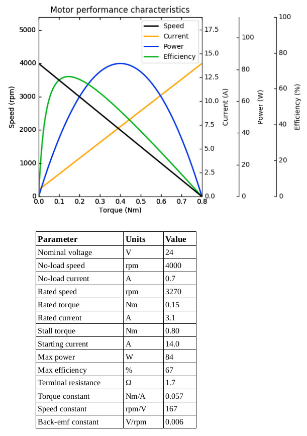
If if you’re not familiar with DC motors, the datasheet above might be overwhelming. By the end of this post, the goal is for us to be able to understand everything on this datasheet. First, let’s break down the performance chart at the top. There are four curves in this chart—speed, current, power, and efficiency—on four different y axes, each plotted against torque on the same x axis. These are called the motor’s “characteristic curves.” It might be easier to examine each curve if we split them up into separate plots:

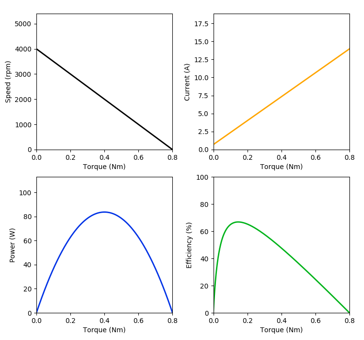
The speed-torque curve in the upper-left is perhaps the most important of these curves. It demonstrates that the relationship between speed and torque is linear. The speed attains a maximum when the torque produced by the motor is zero; this maximum speed is called the “no-load speed,” and is essentially what occurs when nothing is attached to the motor shaft, i.e., there is no load acting against the rotation of the motor and the motor shaft is allowed to spin freely. At the other end of the curve, the speed hits zero and the torque attains a maximum. This is called the “stall torque.”

The current curve, upper-right, demonstrates that the relationship between torque and current draw is also linear. As you might expect, required current increases as torque increases. And, as with speed, the current at zero torque is called the “no-load current.” The other extreme, when the current reaches a maximum, is called the “stall current” or “starting current.” The term “starting current” refers to the fact that, when the motor starts moving from rest, its speed is initially zero and torque is initially at its maximum. The starting current is sometimes also called the “inrush current.” When the motor first starts, it will momentarily draw the maximum amount of current regardless of the physical load attached to the motor shaft, but this inrush only lasts for a small amount of time, usually on the order of milliseconds.

The power curve, lower-left, displays the mechanical power output by the motor. This output power reaches a maximum at exactly half the stall torque, which, as we’ll see in the following sections, is always true. Finally, the efficiency curve, lower-right, illustrates how efficiently the motor converts electrical power to the aforementioned mechanical power.

Basic equations

For our purposes, the motor is governed by two main equations. The first is the conservation of energy (more specifically, the time rate of change of the conservation of energy):

\(P_{electrical} = P_{heat} + P_{mechanical}\) (Equation 1a)

This equation says that the electrical power supplied to the motor is output in the form of dissipated heat and mechanical power. Electrical power is equal to current \(i\) times voltage \(v\). To compute power dissipated as heat, we must keep in mind that the motor’s armature has some resistance \(R\) (the “terminal resistance” on the datasheet), and that the power dissipated by this resistive load is equal to current squared times the resistance. Finally, the mechanical power for a rotating system is given by torque \(\tau\) times angular speed \(\omega\). Rewriting the equation above using these definitions:

\(iv = i^2 R + \tau \omega\) (Equation 1b)

The second main equation is the motor’s voltage balance equation:

\(v = iR + L \frac{di}{dt} + v_\text{emf}\) (Equation 2a)

where \(v\) is the voltage applied to the motor, \(L\) is the inductance of the motor, \(\frac{di}{dt}\) is the instantaneous time rate of change of the current, and \(v_\text{emf}\) is the “back-emf.” First of all, the behavior of a motor depends on the voltage used to drive it. The motor’s characteristic curves (i.e., its no-load speed, stall torque, starting current, etc.) vary based on the voltage. The “nominal voltage” on the datasheet refers to the voltage for which this information is provided. In other words, the characteristic curves and various parameters on the datasheet above are true when the motor is provided a 24V power source (in this example). Generally, you can use a higher or lower voltage to drive the motor, but doing so tends to be less efficient and, if the voltage is too high, risks damaging the motor more quickly due to the larger amount of heat generated. With regard to the inductance \(L\) and the time derivative of current \(\frac{di}{dt}\), we are generally only interested in the behavior of the motor at steady state, i.e., after it’s reached whatever speed/torque we’re interested in. Therefore, we can simply ignore the term \(L \frac{di}{dt}\), because we only care about the behavior of the motor when the current is constant, like so:

\(v = iR + v_{emf}\) (Equation 2b)

Finally, \(v_\text{emf}\) is the back-emf (“emf” stands for electromotive force, which is simply another term for voltage), also known as “counter-emf.” The back-emf is voltage that’s induced by rotation of the motor armature opposite the direction of rotation. In other words, it’s a voltage that acts against the applied voltage (it’s the same effect that allows a motor to be used as a generator). The back-emf is directly proportional to the speed of the motor. The faster the motor spins, the greater the back-emf that must be overcome. The relationship between back-emf and speed is given by the following equation:

\(v_\text{emf} = K_e \omega\) (Equation 3a)

where \(K_e\) is the electrical constant, also known as the “back-emf constant” (which is the last line on the sample datasheet above). Sometimes, the symbol is also written as \(K_b\) for back-emf. This constant relates the back-emf to the speed of the motor. Sometimes, you’ll also see a “speed constant” (like the second to last line of the sample datasheet above); the speed constant \(K_s\) is simply the inverse of the electrical constant:

\(v_\text{emf} = \frac{1}{K_s} \omega\) (Equation 3b)

Sometimes, the speed constant is also called the “velocity constant” and is written \(K_v\).

In addition to the electrical constant and speed constant, both of which relate speed to back-emf, there’s a third constant that relates torque to current—\(K_t\), the torque constant, which is also found on our datasheet above:

\(\tau = K_t i\) (Equation 4)

The torque constant is sometimes also written \(K_m\), where the “m” stands for motor.

The values of these constants depend on the motor, and vary from motor to motor.

There is really just one motor constant!

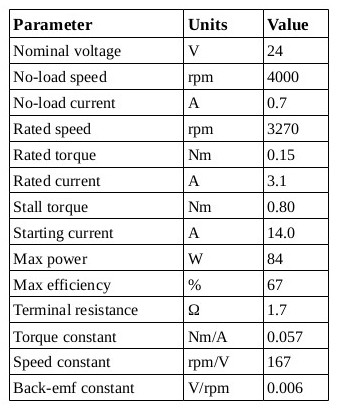
If you’re a fan of vague biblical parallels to engineering topics, then you’re in luck, because these three constants—\(K_e\), \(K_s\), and \(K_t\)—are actually just one constant represented in three different ways. The first two, the electrical constant \(K_e\) and the speed constant \(K_s\), are simply inverses of one another, so the fact that these represent the same constant is fairly obvious. But, it turns out that the third constant, the torque constant \(K_t\), is exactly the same as the electrical constant \(K_e\). They are literally identical to one another. Refer to the motor parameters on the datasheet, which I’ll print again below for convenience:

If the electrical constant (back-emf constant) and the torque constant are identical, why do they have different values on the datasheet? The answer lies in the units. The torque constant is given in Nm/A, whereas the electrical constant is given in V/rpm. Oftentimes, datasheets use rpm rather than SI units of rad/s. If we converted both of these constants to SI units, we would see that they’re equivalent. First, consider Equation 3a again. If we divide through by \(\omega\) to isolate \(K_e\), it would have units of voltage divided by angular speed, which, expressed with rad/s instead of rpm, looks like this:

\[K_e = \frac{v}{\omega} = \frac{V}{(rad/s)} = \frac{V \cdot s}{rad}\]

Then, using the definition of the volt, expressing it in SI units, and recalling that the radian is a dimensionless unit, the above becomes:

\[K_e = \frac{kg \cdot m^2}{A \cdot s^3} \frac{s}{rad} = \frac{kg \cdot m^2}{A \cdot s^2}\]

Similarly, if we divide Equation 4 through by current and write everything in SI units, it looks like this:

\[K_t = \frac{\tau}{i} = \frac{N \cdot m}{A} = \frac{kg \cdot m^2}{A \cdot s^2}\]

If you’re still not convinced, consider Equation 2b, the voltage balance equation. Substituting \(v_\text{emf} = K_e \omega\) from Equation 3a into this results in the following:

\(v = iR + K_e \omega\) (Equation 5a)

Now, consider Equation 1b, the conservation of energy equation, once again. If we divide this equation through by current, we get:

\[v = iR + \frac{\tau}{i} \omega\]

And from Equation 4, \(K_t = \frac{\tau}{i}\). Substituting this into the equation above:

\(v = iR + K_t \omega\) (Equation 5b)

Equations 5a and 5b are equivalent, and show that \(K_e = K_t\). The lesson here, aside from \(K_e = K_t = 1 / K_s\), is to think in SI units regardless of the units the datasheet uses.

Characteristic curves

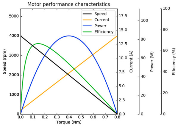
Now that we understand the underlying theory a little better (I hope), let’s investigate where the characteristic curves come from. The performance chart from the datasheet is printed again below for convenience.

Speed

Solving Equation 5b for \(\omega\):

\(\omega = \frac{1}{K_t} (v - iR)\) (Equation 6)

Substituting \(i = \frac{\tau}{K_t}\) from Equation 4 into the equation above:

\[\omega = \frac{1}{K_t} \left(v - \frac{\tau}{K_t}R \right)\]

We can also write this a bit more neatly using the speed constant:

\(\omega = K_s (v - K_s R \tau)\) (Equation 7)

This is the equation of the speed-torque curve. Then, the no-load speed \(\omega_\text{no-load}\) can be found by setting torque equal to zero:

\(\omega_\text{no-load} = K_s v\) (Equation 8)

This tells us that the no-load speed of a motor is directly proportional to the input voltage. We can find the stall torque by setting the speed equal to zero and solving:

\(\tau_\text{stall} = \frac{v}{K_s R}\) (Equation 9)

Notice how the stall torque is also proportional to voltage.

Current

Equation 6 shows that the relationship between speed and current is linear. By extension from the fact that speed and torque are linearly related, we can deduce that torque and current are linearly related as well. Computing the starting current (stall current) is as simple as plugging the stall torque into Equation 4:

\(i_\text{stall} = \frac{\tau_\text{stall}}{K_t} = K_s \tau_\text{stall}\) (Equation 10)**

This might lead us to believe that computing the no-load current \(i_\text{no-load}\) is just a matter of setting torque equal to zero. From the above equation, this would result in a no-load current of zero. However, looking at the current-torque curve in the performance chart, we see that the no-load current, though relatively small, is not zero. This is because, in reality, the motor will always have to overcome friction and inertia even in the absence of additional load on the motor. Therefore, there will always be some current draw at no load, though this no-load current will usually be relatively low.

Power

The power curve is derived from the speed curve. Mechanical power for rotating motion is defined as \(P_\text{mechanical} = \tau \omega\). To write the mechanical power output of the motor in terms of torque, we multiply Equation 7 by torque:

\[P_\text{mechanical} = \tau \omega = \tau [K_s (v - K_s R \tau)] = K_s v \tau - K_s ^2 R \tau^2\]

This expression contains the term \(-\tau^2\), hence why the power curve is an inverted parabola. The motor outputs maximum mechanical power at exactly half the stall torque (or, equivalently, half the no-load speed). If you’re not familiar with calculus, don’t worry—just keep this fact in mind. If you are familiar with calculus, we can see why this is the case by determining the torque at which the power curve attains its maximum, which entails setting the first derivative of the power equation (with respect to torque) equal to zero:

\[\frac{dP_\text{mechanical}}{d\tau} = K_s v - 2K_s^2 R \tau = 0\]

\[2K_s^2 R \tau = K_s v\]

\[\tau = \frac{1}{2} \frac{v}{K_s R}\]

From Equation 9, we know that \(\tau_\text{stall} = \frac{v}{K_s R}\). Therefore, maximum power is always achieved at half this value.

Efficiency

The efficiency curve is derived from the power and current curves, and is defined as:

\[\text{efficiency} = 100\% \times \frac{P_\text{mechanical}}{P_\text{electrical}}\]

The mechanical power at any point along the power curve can be calculated as described in the Power sub-section above. Electrical power is defined as \(P_\text{electrical} = iv\) and can be computed at any point by multiplying the value of the current curve at that point with the voltage. Usually, efficiency peaks at high speed and low torque, as the curve shows us.

Rated (continuous) speed, torque, and current

That leaves the “rated speed,” “rated torque,” and “rated current.” These are sometimes also called “continuous” or “nominal” speed, torque, and current. All of these terms refer to the point along the characteristic curves at which the motor can run continuously without damaging itself. This is based on the thermal characteristics of the motor itself and is not usually something you can compute without more detailed information about the motor. Usually, the rated (or “continuous”/ “nominal”) values happen to be at or near peak efficiency. This makes sense, because the motor produces the least excess heat at peak efficiency.

However, not all applications require continuous operation, which is also known as a 100% duty cycle. Maybe for your application, your motor will only have to be on 30% of the time (i.e., a 30% duty cycle). In this case, you would probably be able to safely operate at a higher torque/lower speed/higher current. This depends largely on the motor, though, so if you’re unsure and it’s important for your application, your best bet is to contact the manufacturer for more information (or test the motor and see if it meets your requirements).

What if the datasheet only provides some information?

Not all motor datasheets will contain all of this information. At a bare minimum, though, you’ll usually be given the no-load speed, stall torque, and nominal voltage. This is enough information to get solid estimates for everything else. You can use the no-load speed and nominal voltage with Equation 8 to determine the motor constants. Then you can use the stall torque, nominal voltage, and motor constant with Equation 9 to compute the terminal resistance. To determine the stall current, use the stall torque and motor constant with Equation 10. No-load current will vary depending on the motor but, usually, you can assume it will be relatively low. From there, you can construct the power and efficiency curves as described in the previous section.

Conclusion

If you’ve gotten through this, you should, hopefully, have a better understanding of the information presented on DC motor datasheets. Try rereading the sample datasheet and ensure, if you couldn’t interpret everything on it before, that you can do it now. Of course, being able to read a motor datasheet is just one aspect of selecting a motor. Selecting a motor also requires one to know the requirements for whatever application the motor is being used in. This is another topic in itself, and may be covered in future posts.