In the last post, we covered 2D rotation matrices, which allow us to convert coordinates from one coordinate system to another coordinate system that's rotated by some angle \(\theta\). Previously, we notated the original coordinate system \(XY\) and the rotated coordinate system \(X'Y'\). In this post, we'll begin dealing with a larger number of coordinate systems. Adding a prime for each additional coordinate system would be impractical and inconvenient, so we'll use numerical subscripts to differentiate between coordinate systems, instead.
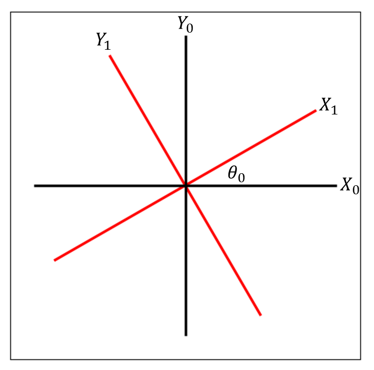
Referring to the image above, the \(X_0Y_0\) coordinate system is equivalent to the \(XY\) coordinate system from the previous post, and will generally represent the “global” coordinate system we're most interested in. The \(X_1Y_1\) coordinate system is equivalent to the \(X'Y'\) coordinate system from the previous post, and \(\theta_0\) is equivalent to \(\theta\). The rotation matrix to convert from the \(X_1Y_1\) system to the \(X_0Y_0\) system would be
\[ [R] = \left[ \begin{matrix} \cos{\theta_0} & -\sin{\theta_0} \\ \sin{\theta_0} & \cos{\theta_0} \end{matrix} \right] \]
Converting a vector defined in the \(X_1Y_1\) system to the \(X_0Y_0\) system would look like this:
\[ \left\{ \begin{matrix} x_0 \\ y_0 \end{matrix} \right\} = \left[ \begin{matrix} \cos{\theta_0} & -\sin{\theta_0} \\ \sin{\theta_0} & \cos{\theta_0} \end{matrix} \right] \left\{ \begin{matrix} x_1 \\ y_1 \end{matrix} \right\} \]
A Euclidean transformation matrix that can perform both rotation and translation looks similar to this, but contains an additional row and and an additional column:
\[ [T] = \left[ \begin{matrix} \cos{\theta_0} & -\sin{\theta_0} & 0 \\ \sin{\theta_0} & \cos{\theta_0} & 0 \\ 0 & 0 & 1 \end{matrix} \right] \]
The last column of the first row provides the translation in x along the \(X_0\) axis, and the last column of the second row provides the translation in y along the \(Y_0\) axis. For pure rotation without translation, these elements are equal to zero. The last row of the transformation matrix always contains zeros except for the final element, which is always a one. Similarly, the position vector for a point intended to be used with a transformation matrix must contain an additional dummy coordinate that's always equal to one:
\[ \left\{ \begin{matrix} x_0 \\ y_0 \\ 1 \end{matrix} \right\} = \left[ \begin{matrix} \cos{\theta_0} & -\sin{\theta_0} & 0 \\ \sin{\theta_0} & \cos{\theta_0} & 0 \\ 0 & 0 & 1 \end{matrix} \right] \left\{ \begin{matrix} x_1 \\ y_1 \\ 1 \end{matrix} \right\} \]
Consider an example where there is translation, say, for instance, some distance \(a\) along \(X_0\) and some distance \(b\) along \(Y_0\):
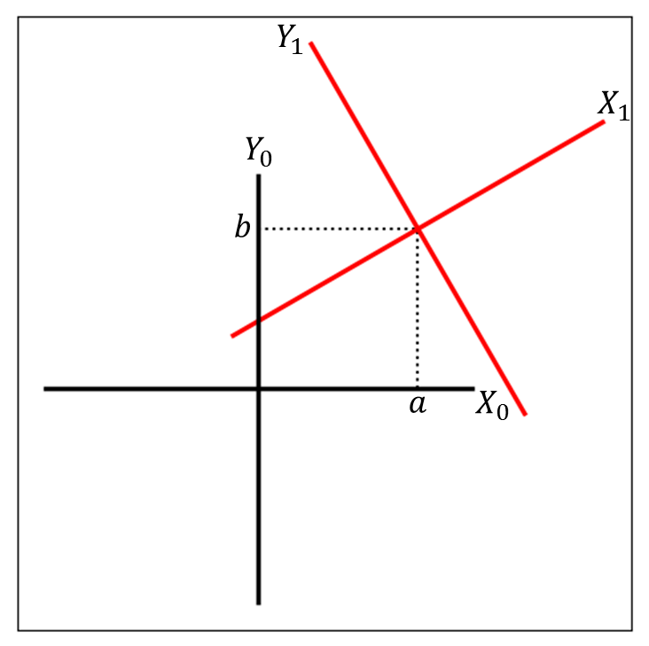
The equation and transformation matrix in this case would be
\[ \left\{ \begin{matrix} x_0 \\ y_0 \\ 1 \end{matrix} \right\} = \left[ \begin{matrix} \cos{\theta_0} & -\sin{\theta_0} & a \\ \sin{\theta_0} & \cos{\theta_0} & b \\ 0 & 0 & 1 \end{matrix} \right] \left\{ \begin{matrix} x_1 \\ y_1 \\ 1 \end{matrix} \right\} \]
If it's not apparent why this is the case, try working through the matrix multiplication to see how these additional elements affect the resulting coordinates. A simple example to consider might be
\[ \left\{ \begin{matrix} x_1 \\ y_1 \\ 1 \end{matrix} \right\} = \left\{ \begin{matrix} 0 \\ 0 \\ 1 \end{matrix} \right\} \]
i.e., the origin of the second coordinate system, for which you should simply obtain \(x_0 = a\) and \(y_0 = b\).
The true value in using transformation matrices is the ability to chain together multiple transformation matrices. In other words, if you have one coordinate system that's defined in another coordinate system (by its rotation and translation relative to that other coordinate system), which, in turn, is defined in yet another coordinate system, and so on, you can obtain the coordinates of some point in the desired coordinate system by multiplying the transformation matrices of all the intervening coordinate systems. For example, consider the following case, which contains three coordinate systems:
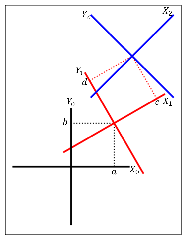
Here, the \(X_1Y_1\) system (drawn in red) is defined by its rotation and translation relative to the \(X_0Y_0\) system (drawn in black), specifically:
\[ \left[ ^0 T_1 \right] = \left[ \begin{matrix} \cos{\theta_0} & -\sin{\theta_0} & a \\ \sin{\theta_0} & \cos{\theta_0} & b \\ 0 & 0 & 1 \end{matrix} \right] \]
where the notation on the left-hand side indicates that the transformation matrix is converting from the \(X_1Y_1\) system to the \(X_0Y_0\) system. Further, the \(X_2Y_2\) system (drawn in blue) is defined by its rotation (by some angle \(\theta_1\)) and translation (\(c\) in the \(X_1\) direction and \(d\) in the \(Y_1\) direction) relative to the \(X_1Y_1\) system, i.e.:
\[ \left[ ^1 T_2 \right] = \left[ \begin{matrix} \cos{\theta_1} & -\sin{\theta_1} & c \\ \sin{\theta_1} & \cos{\theta_1} & d \\ 0 & 0 & 1 \end{matrix} \right] \]
To convert coordinates from the \(X_2Y_2\) system to the \(X_0Y_0\) system, the transformation matrices are successively multiplied:
\[ \left[ ^0 T_2 \right] = \left[ ^0 T_1 \right] \left[ ^1 T_2 \right] \]
If it's not clear why this works, consider the following example. Let's say we have some position vector defined in the \(X_2Y_2\) system, which we'll write as \(\mathbf{r_2}\), and we'd like to obtain its coordinates in terms of the \(X_0Y_0\) system, which we'll write as \(\mathbf{r_0}\). This is the same as writing:
\[ \mathbf{r_0} = \left[ ^0 T_1 \right] \left[ ^1 T_2 \right] \mathbf{r_2} \]
The term \(\left[ ^1 T_2 \right] \mathbf{r_2}\) on the right-hand side just says “convert the coordinates \(\mathbf{r_2}\) from the \(X_2Y_2\) system to the \(X_1Y_1\) system,” i.e., \(\mathbf{r_1} = \left[ ^1 T_2 \right] \mathbf{r_2}\). Then, to convert \(\mathbf{r_1}\) to \(\mathbf{r_0}\), we multiply by \(\left[ ^0 T_1 \right]\). Note that the order in which we multiply the transformation matrices matters—matrix multiplication is not commutative, and multiplying them in the wrong order will affect the result.
Let's look at a concrete example to attain some intuition for how to apply these concepts. Suppose we have a robot arm with two segments, each controlled by a revolute joint. At the end of the second segment is the robot arm's end effector—this end effector might be some sort of claw, manipulator, or gripper that's designed to grab things.
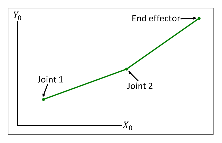
You can liken this to a human arm, where joint 1 would be the shoulder, joint 2 would be the elbow, and the end effector would be the hand. Knowing only the length of each segment (which will always remain constant) and the angular displacement of each joint (which we might control using motors), how can we determine the position of the end effector in 2D space? In this example, joint 1 (the “shoulder joint”) isn't necessarily located at the center of our primary coordinate system, but is offset by some distance in \(X_0\) and \(Y_0\).
One way to approach this is to define a coordinate system at each joint. The \(X_1Y_1\) system at the first joint is offset from the \(X_0Y_0\) system by an angle \(\theta_0\), a distance \(a\) in \(X_0\), and a distance \(b\) in \(Y_0\):
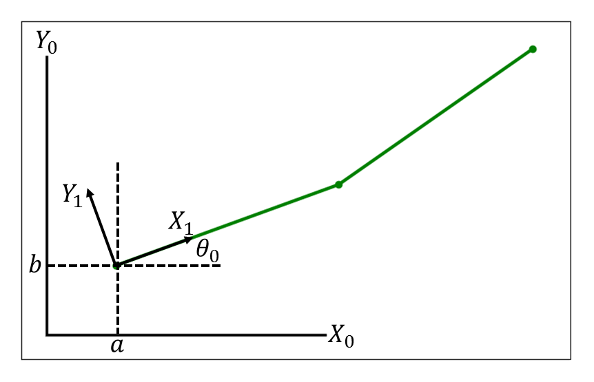
where \(\theta_0\) corresponds to the angular displacement of the joint, and the first segment is aligned with the \(X_1\) axis. The transformation matrix for this coordinate system is
\[ \left[ ^0 T_1 \right] = \left[ \begin{matrix} \cos{\theta_0} & -\sin{\theta_0} & a \\ \sin{\theta_0} & \cos{\theta_0} & b \\ 0 & 0 & 1 \end{matrix} \right] \]
We might then define the next coordinate system, \(X_2Y_2\), to be located at the second joint a distance \(c\) along the \(X_1\) axis (i.e., the first segment, or the “upper arm,” is of length \(c\)), and offset by a rotation \(\theta_1\) corresponding to the angular displacement of the second joint.
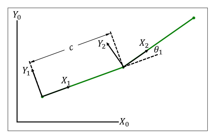
The transformation matrix for this \(X_2Y_2\) system, relative to the \(X_1Y_1\) system, is
\[ \left[ ^1 T_2 \right] = \left[ \begin{matrix} \cos{\theta_1} & -\sin{\theta_1} & c \\ \sin{\theta_1} & \cos{\theta_1} & 0 \\ 0 & 0 & 1 \end{matrix} \right] \]
Note that the offset in \(Y_1\) is zero, since the coordinate system is positioned in line with the the “upper arm” along \(X_1\). Finally, suppose that the length of the second segment (the “forearm”), which lies along \(X_2\), is \(d\).
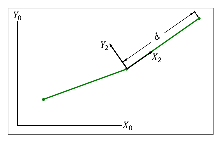
Then the coordinates of the end effector in the \(X_2Y_2\) system, \(\mathbf{r_2}\), are given by
\[ \mathbf{r_2} = \left\{ \begin{matrix} d \\ 0 \\ 1 \end{matrix} \right\} \]
Remember that we want the coordinates of the end effector in the \(X_0Y_0\) system, i.e., \(\mathbf{r_0}\). We obtain this by multiplying the position vector from the \(X_2Y_2\) system by the transformation matrices in the correct order:
\[ \mathbf{r_0} = \left[ ^0 T_1 \right] \left[ ^1 T_2 \right] \mathbf{r_2} \]
Or, writing the right-hand side out in full:
\[ \mathbf{r_0} = \left[ \begin{matrix} \cos{\theta_0} & -\sin{\theta_0} & a \\ \sin{\theta_0} & \cos{\theta_0} & b \\ 0 & 0 & 1 \end{matrix} \right] \left[ \begin{matrix} \cos{\theta_1} & -\sin{\theta_1} & c \\ \sin{\theta_1} & \cos{\theta_1} & 0 \\ 0 & 0 & 1 \end{matrix} \right] \left\{ \begin{matrix} d \\ 0 \\ 1 \end{matrix} \right\} \]
Carrying out the matrix multiplication is left as an exercise for you, the reader.
There you have it—a crash course in Euclidean transformation matrices. If some of these concepts haven't quite stuck, you may want to reread the post, working through the examples with pen and paper until you've internalized them. If you're comfortable with 2D Euclidean transformations, consider reading up on 3D Euclidean transformations, if you're not already familiar with them. These topics will likely be revisited and applied in future posts.
