In the past, I’ve found myself having to (or, at least, really wanting to) draw and animate a clean-looking 2D spring between any two arbitrary points. This post from January, in which I represented the suspension struts of a car with 2D springs in matplotlib, is a notable example. Unable to find a good existing tool for plotting a spring, I decided to make my own. Here’s a demo of it in action:

If you’re electronically inclined, it doubles as a resistor symbol (though I don’t think a resistor that extends and compresses is what they mean by “variable resistor”).

The code for the spring() function that produces the x and y coordinates of each point of the spring can be found on my Github.

The math

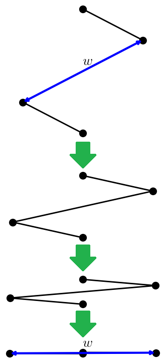
If a picture is worth a thousand words, an equation must be worth at least a hundred. In this section, we’ll combine the two to briefly examine how the function works. First, let’s define the spring as a sawtooth-shaped set of lines between two endpoints. Because this looks like a series of points or nodes connected by lines, I’ve elected to refer to the points as “nodes” (each node can be thought of as a spring coil).

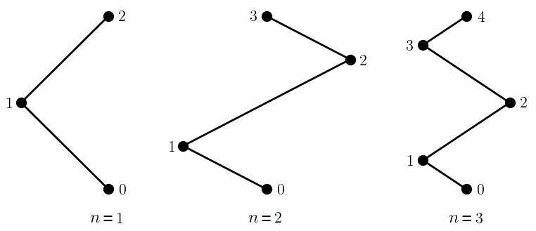
We’ll use \(n\) to describe the number of nodes between the two endpoints (counting the endpoints, any given spring will have \(n+2\) nodes numbered from \(0\) to \(n+1\)). The figure above shows what springs with \(n=1\), \(n=2\), and \(n=3\) nodes look like and how the nodes are numbered (node \(0\) is the first endpoint and node \(n+1\) is the other endpoint). These figures illustrate the case where both endpoints are aligned vertically for simplicity, but the endpoints can be anywhere in space.

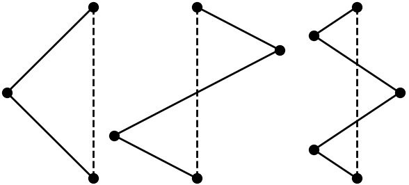
Observe the pattern in the figure above—starting at node \(0\), the next node is offset some perpendicular distance from the imaginary centerline between the endpoints and some parallel distance along the centerline; the node after that is offset the same perpendicular distance in the other direction and some multiple of the parallel distance along the centerline. Here’s what that centerline would look like for each example:

Next, let’s define the distance, or length, between the two endpoints as \(l\), i.e., the length of the centerline.

Using this distance and the aforementioned pattern, the following relationship based on the distance \(l\) between the endpoints and the number of nodes \(n\) between the endpoints emerges:

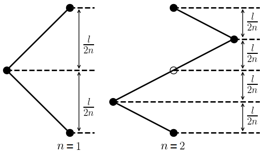
In this figure, \(n=1\) and \(n=2\) are used as representative examples, but the same pattern can be observed for any values of \(l\) and \(n\). After the root node (node \(0\)), each subsequent node \(i\) is located a specific distance along the centerline, given by the following expression:

\(\displaystyle (d_i)_{\parallel} = \frac{l}{2n}(2i - 1)\) (Equation 1)

where \((d_i)_{\parallel}\) refers to the distance of the \(i^\text{th}\) node along (parallel to) the centerline, excluding the endpoints. In other words, node \(1\) is located a distance \(\displaystyle\frac{l}{2n}(2(1)-1) = \frac{l}{2n}\) along the centerline, node \(2\) is located a distance \(\displaystyle\frac{l}{2n}(2(2)-1) = \frac{3l}{2n}\) along the centerline, and so on.

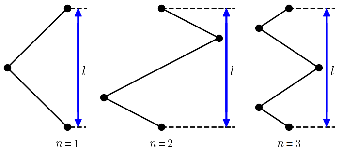
Now, let’s define the width \(w\) of the spring, which is essentially the length of each full line between nodes and can also be thought of as the diameter of the spring. This is, perhaps, best illustrated by the figure adjacent, which shows how each “link” in the spring moves as the spring compresses or extends. When the spring is fully compressed, i.e., when the two endpoints are on top of each other, \(w\) is the width (or diameter) of the spring, at which position the nodes (not counting the endpoints) are a perpendicular distance \(\displaystyle \frac{w}{2}\) from the center of the spring.

Because \(w\) is fixed, the actual perpendicular distance of each node from the centerline of the spring will be lower when the spring is stretched. The actual distance can be determined using the Pythagorean theorem, shown in the figure below.

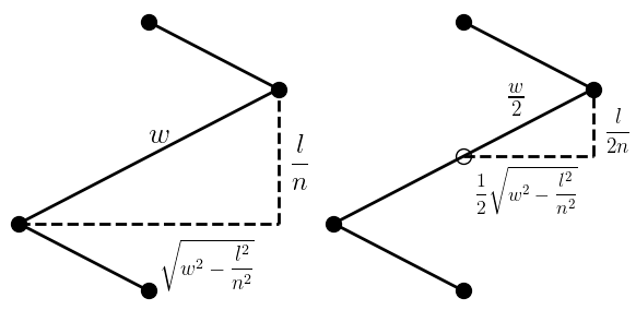
In the figure above, I’ve shown the right-triangle relationship for both an entire line and for half a line. We really only care about the half-line, since we want the perpendicular distance of each node from the centerline, not from the previous node. Again, observe the pattern. Each node will be a perpendicular distance \(\displaystyle \frac{1}{2} \sqrt{w^2 - \frac{l^2}{n^2}}\) from the centerline, alternating between the two sides of the centerline. In other words:

\(\displaystyle (d_i)_{\perp} = \frac{1}{2}\sqrt{w^2 - \frac{l^2}{n^2}}(-1)^i\) (Equation 2)

where \((d_i)_{\perp}\) is the distance of the \(i\mathrm{th}\) node from (perpendicular to) the centerline, excluding the endpoints.

There’s a potential pitfall here if we’re not careful—notice that the spring can extend to a maximum length of \(nw\), at which point it would just be a straight line. If \(l > nw\), the spring can’t physically attain the necessary length because the quantity inside the square root \( \sqrt{w^2 – \frac{l^2}{n^2}}\) is negative.

The last step involves computing the unit vectors tangent (parallel) to and normal (perpendicular) to the centerline between the endpoints in order to generate a spring between any two arbitrary endpoints, regardless of how they’re oriented in space:

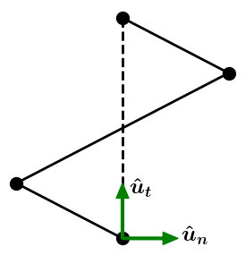
The unit tangent (parallel) vector is computed as the difference of the positions of the two endpoints divided by the distance between them:

\(\displaystyle \hat{\mathbf{u}}_t = \frac{\mathbf{r}_{n+1} - \mathbf{r}_0}{l}\) (Equation 3)

where \(\mathbf{r}_0\) is the position (x and y coordinates) of the first endpoint, \(\mathbf{r}_{n+1}\) is the position of the second endpoint, and \(l\) is the previously defined distance between them, i.e., \(l = \| \mathbf{r}_{n+1} - \mathbf{r}_0 \|\).

To obtain \(\hat{\mathbf{u}}_n\), which is perpendicular to \(\hat{\mathbf{u}}_t\), we can simply swap the x and y coordinates of \(\hat{\mathbf{u}}_t\) and arbitrarily negate one of them. Because I have a potentially unhealthy appreciation for linear algebra, we can write this as follows with a simple 2×2 matrix:

\(\displaystyle \hat{\mathbf{u}}_n = \begin{bmatrix} 0 & -1 \\ 1 & 0 \end{bmatrix} \hat{\mathbf{u}}_t\) (Equation 4)

Finally, to obtain the absolute position of each node between the endpoints, we combine Equation 1, Equation 2, Equation 3, and Equation 4 and add them to the position of the first endpoint:

\(\displaystyle \mathbf{r}_i = \mathbf{r}_0 + \frac{l}{2n}(2i-1)\hat{\mathbf{u}}_t + \frac{1}{2}\sqrt{w^2 - \frac{l^2}{n^2}}(-1)^i \hat{\mathbf{u}}_n\) (Equation 5)

The code

The code can be found on Github. The spring() function takes the arguments start (the first endpoint \(\mathbf{r}_0\)), end (the second endpoint \(\mathbf{r}_{n+1}\)), nodes (the number of intermediate nodes \(n\)), and width (the width \(w\)). start and end may be 2-tuples, or numpy arrays of 2 elements, etc.

 4
 5
 6
 7
 8
 9
10
11
12

def spring(start, end, nodes, width):
    """!
    Return a list of points corresponding to a spring.
    @param r1 (array-like) The (x, y) coordinates of the first endpoint.
    @param r2 (array-like) The (x, y) coordinates of the second endpoint.
    @param nodes (int) The number of spring "nodes" or coils.
    @param width (int or float) The diameter of the spring.
    @return An array of x coordinates and an array of y coordinates.
    """

Line 16 ensures that a positive non-zero integer number of nodes is chosen.

16

nodes = max(int(nodes), 1)

After computing the length and the tangent and normal unit vectors, we’ll initialize a \(2 \times (n+2)\) numpy array of all the points in sequence, where the first row corresponds to the x coordinates, the second to the y coordinates, and each column to a point. The first endpoint is assigned to the first column and the other endpoint is assigned to the last column.

30
31

spring_coords = np.zeros((2, nodes + 2))
spring_coords[:,0], spring_coords[:,-1] = start, end

On line 36, the magnitude of the normal (perpendicular) distance of the nodes from the centerline, from Equation 2, is calculated, taking care to account for the case where the quantity in the square root is negative, in which case the value is set to 0, forming a straight line.

36

normal_dist = math.sqrt(max(0, width**2 - (length**2 / nodes**2))) / 2

Lastly, we iterate through nodes \(1\) to \(n\), applying Equation 5 to compute the coordinates of each point.

39
40
41
42
43
44
45

for i in range(1, nodes + 1):
    spring_coords[:,i] = (
        start
        + ((length * (2 * i - 1) * u_t) / (2 * nodes))
        + (normal_dist * (-1)**i * u_n))

return spring_coords[0,:], spring_coords[1,:]

I’ve opted to return each row (x coordinates and y coordinates) separately, making it easy to feed the output of the function to matplotlib.pyplot.plot() or to the set_data() method of an existing matplotlib Line2D object on each iteration of an animation.

Hope you’ve found this post or the tool to be helpful!