Path-planning, as the name suggests, is the process of determining how to get from one point to another. Path-planning, also called motion planning, has applications in a number of fields, like autonomous robotics and GPS navigation, to name a couple. Before getting into the heart of the matter, let’s start with a demonstration of the Python script and interactive plot we’re going to have up and running by the end of this post:

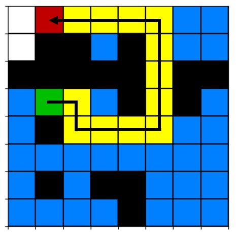
As you can see from the video, we’re going to learn about and implement a path-planning algorithm that tries to find the shortest path (yellow) on a grid from a start cell (the green square) to a destination cell (the red square) while navigating around obstacles (the black cells). Read on for the details.

Graph-based path-planning

There exist a number of techniques and algorithms for path-planning, one of which includes graph-based methods. In graph theory, a graph is defined as a structure consisting of “nodes,” i.e., points, and “edges,” i.e., lines that connect the nodes. In graph-based path-planning, we travel from node to node along the edges, with the aim of figuring out how to get from some initial node to a destination node.

We’re going to examine a particular type of graph: the grid, also known as a lattice graph. Each cell of our grid can be thought of as a node, and the path between each node can be thought of as an edge. The defining characteristic of a grid is that all the edges are the same length. In this post, we’ll be working with a square grid.

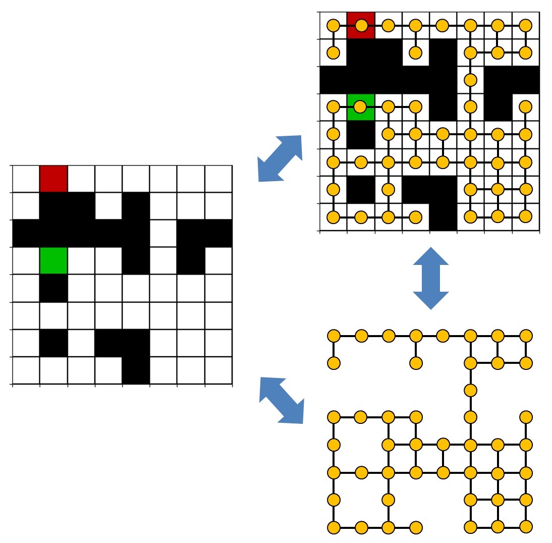
In the figure above, left, we see our grid, which looks kind of like a crossword puzzle. The white squares represent empty cells to which we can travel. The black squares are obstacles. The green square is the start cell, and the red square is the destination cell. In the figure, top right, the graph representation of the grid is superimposed on the grid. Each orange dot is a node, and the lines between nodes are edges. In the figure, bottom right, I’ve isolated the graph representation to get a better look at it. Notice how the nodes are connected—from any given node, it’s only possible to travel up, down, right, or left, not diagonally. We don’t have to limit ourselves to this, of course. If we wanted to, we could also define our grid to have diagonal edges between nodes, but we’ll keep things simple for this example.

Finding the shortest path

Our goal will be to find the shortest path from the start cell to the destination cell. A number of methods exist to get from start to finish, including depth-first search, which follows a single path until it either finds the destination or, more likely, hits a dead-end, at which point it backtracks to the last fork in the road and follows a different path—repeat until the destination is found or until there are no paths left to explore. However, this is not guaranteed to find the shortest path, only to find a path if one exists. Another method is the breadth-first search, which explores evenly out from the start cell and is guaranteed to find the shortest path. One of the simplest types of breadth-first search algorithms, which we saw in the video at the beginning of this post, is sometimes referred to as the wavefront or grassfire algorithm, so named because the search path looks like a spreading shockwave or brush fire. The idea behind the algorithm is to mark each cell (node) with its distance from the start cell, exploring the cells adjacent to all cells at the current depth (distance) before moving on to the next depth:

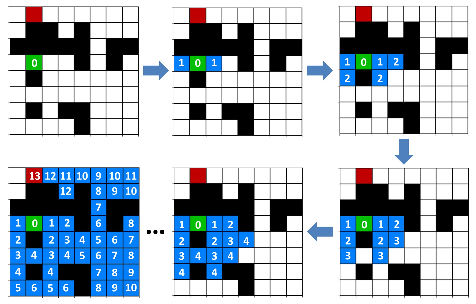
First, we mark our start cell with “0” (see figure above, top left). Then, we look at the cells above, below, to the right, and to the left of the start cell. We mark each of the cells in those directions with a “1”, assuming they’re not obstacles or outside the boundaries of the grid, because they’re 1 step away from the start cell. Since there’s only one cell with a depth of “0”, the start cell, that’s it for the first iteration. On the next iteration, we consider each cell marked with depth “1” and look at the cells adjacent to those, then mark them with “2” to indicate that they’re 2 steps away from the start cell. We continue in this manner, only marking adjacent cells with the next depth if they’re not already marked with a smaller number, which would indicate that they’re already closer to the start cell than the current cell. This process continues until either a) the destination is found or b) all reachable cells have been explored and no path to the destination exists. If the destination is found, we can backtrack to find the shortest path by following the cells in reverse numerical order back to the start cell:

Note that, in our implementation of the algorithm, backtracking will be arbitrary—if there are multiple shortest paths, our algorithm will only choose one of them.

The code, part 1

To implement and animate the algorithm, we’ll create two files, both available on Github: Grassfire.py animGrassfire.py

First, create a file named Grassfire.py (or get it from the Github link above).

 1
 2
 3
 4
 5
 6
 7
 8
 9
10
11
12
13
14
15
16
17

import numpy as np
import random
import math

PI = math.pi

class Grassfire:
    '''Class is a container for constants and methods we'll use
        to create, modify, and plot a 2D grid of pixels
        demonstrating the grassfire path-planning algorithm.
    '''

    START = 0
    DEST = -1     # destination
    UNVIS = -2    # unvisited
    OBST = -3     # obstacle
    PATH = -4

After taking care of our imports and defining pi as a constant, we define a class we’ll call Grassfire. We’ll use the variables and methods in this class to create and manipulate our grid, as well as to execute the Grassfire algorithm. Our grid will be 2D numpy integer array. As discussed above, we’ll utilize 0 to denote the start cell and positive integers to indicate the distance of visited cells from the start cell. The negative integers on lines 14-17 are reserved for, respectively: the destination, unvisited cells, obstacles, and cells that are part of the shortest path if the destination is found. Note that these are class variables (which we’re treating as constants), meaning that they are shared across all instances of a class.

19
20
21
22
23
24
25
26

# Each of the above cell values is represented by an RGB color
# on the plot. COLOR_VIS refers to visited cells (value > 0).
COLOR_START = np.array([0, 0.75, 0])
COLOR_DEST = np.array([0.75, 0, 0])
COLOR_UNVIS = np.array([1, 1, 1])
COLOR_VIS = np.array([0, 0.5, 1])
COLOR_OBST = np.array([0, 0, 0])
COLOR_PATH = np.array([1, 1, 0])

In addition to the main grid, which contains the locations of the start and destination, obstacles, distances of visited cells, etc., we’ll also need a corresponding grid that translates that information into colors. This colorGrid will simply be an RGB pixel map, with each pixel representing one cell of our grid. If the main grid has dimensions MxN, then the colorGrid will have dimensions MxNx3, where the third axis contains the RGB values for each cell. Lines 21-26 define the RGB colors for each cell type.

28
29
30
31
32
33
34
35
36
37
38
39

def random_grid(self, rows=16, cols=16, obstacleProb=0.3):
    '''Return a 2D numpy array representing a grid of randomly placed
    obstacles (where the likelihood of any cell being an obstacle
    is given by obstacleProb) and randomized start/destination cells.
    '''
    obstacleGrid = np.random.random_sample((rows, cols))
    grid = Grassfire.UNVIS * np.ones((rows, cols), dtype=np.int)
    grid[obstacleGrid <= obstacleProb] = self.OBST

    # Randomly set start and destination cells.
    self.set_start_dest(grid)
    return grid

The random_grid() method is the only method in our class that actually returns a fresh, randomized grid. Observe that we prefix class attributes (variables) with the class name, e.g., Grassfire.UNVIS. We use the numpy function random_sample() to generate an array of floats from 0 to 1, obstacleGrid. On line 34, we initialize our main grid, grid, to an array representing unvisited cells. Since obstacleGrid and grid have the same dimensions, we find the values of obstacleGrid less than our obstacle probability threshold and set those elements in grid to be obstacles on line 35. The comparative statement obstacleGrid <= obstacleProb produces a Boolean array of the same size as obstacleGrid, where elements satisfying the condition are True and the rest are False. Since this Boolean array is also the same size as grid, we can use it to index into grid and modify only those elements where the condition is True.

Finally, on line 38, we use the method set_start_dest(), which we’ll define next, to randomly select start and destination locations. Note that we supply the set_start_dest() method with grid without an assignment and without worrying about the return value of set_start_dest(). In other words, notice how we didn’t write line 38 as grid = self.set_start_dest(grid). That’s because numpy arrays are passed by reference, not by value. This means that passing grid to a function doesn’t pass a copy of grid —instead, it passes a reference to the original array itself, so that any changes set_start_dest() makes to grid are made to the original array.

41
42
43
44
45
46
47
48
49
50
51
52
53
54
55
56
57
58
59
60
61
62
63
64
65

def set_start_dest(self, grid):
    '''For a given grid, randomly select start and destination cells.'''
    (rows, cols) = grid.shape

    # Remove existing start and dest cells, if any.
    grid[grid == Grassfire.START] = Grassfire.UNVIS
    grid[grid == Grassfire.DEST] = Grassfire.UNVIS

    # Randomize start cell.
    validStartCell = False
    while not validStartCell:
        startIndex = random.randint(0, rows * cols - 1)
        startIndices = np.unravel_index(startIndex, (rows, cols))
        if grid[startIndices] != Grassfire.OBST:
            validStartCell = True
            grid[startIndices] = Grassfire.START

    # Randomize destination cell.
    validDestCell = False
    while not validDestCell:
        destIndex = random.randint(0, rows * cols - 1)
        destIndices = np.unravel_index(destIndex, (rows, cols))
        if grid[destIndices] != Grassfire.START and grid[destIndices] != Grassfire.OBST:
            validDestCell = True
            grid[destIndices] = Grassfire.DEST

In the method set_start_dest(), we use the function random.randint() to select a random integer within the range of the total number of cells in our grid. This single integer is essentially a flattened index, i.e., the index of an element in the grid if the 2D grid were flattened into a 1D array by arranging all the rows next to one another. The numpy function unravel_index() takes this 1D index and converts it into a pair of 2D indices (note that the function can be used to convert an index into a set of indices in any number of dimensions, not just two dimensions).

67
68
69
70
71
72
73
74
75
76
77
78
79
80
81
82
83
84

def color_grid(self, grid):
    '''Return MxNx3 pixel array ("color grid") corresponding to a grid.'''
    (rows, cols) = grid.shape
    colorGrid = np.zeros((rows, cols, 3), dtype=np.float)

    colorGrid[grid == Grassfire.OBST, :] = Grassfire.COLOR_OBST
    colorGrid[grid == Grassfire.UNVIS, :] = Grassfire.COLOR_UNVIS
    colorGrid[grid == Grassfire.START, :] = Grassfire.COLOR_START
    colorGrid[grid == Grassfire.DEST, :] = Grassfire.COLOR_DEST
    colorGrid[grid > Grassfire.START, :] = Grassfire.COLOR_VIS
    colorGrid[grid == Grassfire.PATH, :] = Grassfire.COLOR_PATH
    return colorGrid

def reset_grid(self, grid):
    '''Reset cells that are not OBST, START, or DEST to UNVIS.'''
    cellsToReset = ~((grid == Grassfire.OBST) + (grid == Grassfire.START)
        + (grid == Grassfire.DEST))
    grid[cellsToReset] = Grassfire.UNVIS

As we discussed above, the function color_grid() returns an RGB pixel array to visually represent grid. In the reset_grid() method, lines 82-83 demonstrate that Boolean arrays can be added to one another.

Finally, we’ll define the methods that actually implement the algorithm, beginning with two helper methods followed by the main pathfinding method. On each iteration, our implementation of the algorithm will check the cells adjacent to every cell matching the current depth. If any of these adjacent cells are unvisited or have a value greater than the current depth + 1, they will be updated to a value of current depth + 1 (indicating that they’re 1 step farther from the start cell than cells of the current depth). We will keep track of how many adjacent cells are updated during each iteration; if, after going through all cells at the current depth, the number of updated cells is 0, it means we’ve explored all visitable cells that can be reached and that no path to the destination exists. During this process, we’ll also be checking to see if the destination is found.

 86
 87
 88
 89
 90
 91
 92
 93
 94
 95
 96
 97
 98
 99
100
101
102
103
104
105
106
107
108
109
110
111
112
113
114
115
116
117
118

def _check_adjacent(self, grid, cell, currentDepth):
    '''For given grid, check the cells adjacent to a given
        cell. If any have a depth (positive int) greater
        than the current depth, update them with the current
        depth, where depth represents distance from start cell.
        If destination found, return DEST constant; else, return
        number of adjacent cells updated.
    '''
    (rows, cols) = grid.shape

    # Track how many adjacent cells are updated.
    numCellsUpdated = 0

    # From the current cell, examine, using sin and cos:
    # cell to right (col + 1), cell below (row + 1),
    # cell to left (col - 1), cell above (row - 1).
    for i in range(4):
        rowToCheck = cell[0] + int(math.sin((PI/2) * i))
        colToCheck = cell[1] + int(math.cos((PI/2) * i))

        # Ensure cell is within bounds of grid.
        if not (0 <= rowToCheck < rows and 0 <= colToCheck < cols):
            continue
        # Check if destination found.
        elif grid[rowToCheck, colToCheck] == Grassfire.DEST:
            return Grassfire.DEST
        # If adjacent cell unvisited or depth > currentDepth + 1,
        # mark with new depth.
        elif (grid[rowToCheck, colToCheck] == Grassfire.UNVIS
            or grid[rowToCheck, colToCheck] > currentDepth + 1):
            grid[rowToCheck, colToCheck] = currentDepth + 1
            numCellsUpdated += 1
    return numCellsUpdated

First, the helper method _check_adjacent() which, given a grid and a cell within the grid, checks the four cells adjacent to the given cell. Note the use of sine and cosine to achieve this compactly. Also observe how, in Python, we can write comparative statements like 0 <= rowToCheck < rows instead of splitting them into two statements.

120
121
122
123
124
125
126
127
128
129
130
131
132
133
134
135
136
137

def _backtrack(self, grid, cell, currentDepth):
    '''This function is used if the destination is found. Similar
        to _check_adjacent(), but returns coordinates of first
        surrounding cell whose value matches "currentDepth", ie,
        the next cell along the path from destination to start.
    '''
    (rows, cols) = grid.shape

    for i in range(4):
        rowToCheck = cell[0] + int(math.sin((PI/2) * i))
        colToCheck = cell[1] + int(math.cos((PI/2) * i))

        if not (0 <= rowToCheck < rows and 0 <= colToCheck < cols):
            continue
        elif grid[rowToCheck, colToCheck] == currentDepth:
            nextCell = (rowToCheck, colToCheck)
            grid[nextCell] = Grassfire.PATH
            return nextCell

The second helper method, _backtrack(), is similar to the previous method, except it modifies the first matching adjacent cell to the value given by the PATH constant, then returns a tuple containing the row and column of the modified cell. The modified cell will be used as the input to the next call of _backtrack(). This will repeat until we’ve arrived back at the start cell.

139
140
141
142
143
144
145
146
147
148
149
150
151
152
153
154
155
156
157
158
159
160
161
162
163
164
165
166
167
168
169
170
171
172
173
174
175
176
177
178
179
180

def find_path(self, grid):
    '''Execute grassfire algorithm by spreading from the start cell out.
        If destination is found, use _backtrack() to trace path from
        destination back to start. Returns a generator function to
        allow stepping through and animating the algorithm.
    '''
    nonlocalDict = {'grid': grid}
    def find_path_generator():
        grid = nonlocalDict['grid']
        depth = 0
        destFound = False
        cellsExhausted = False

        while (not destFound) and (not cellsExhausted):
            numCellsModified = 0
            depthIndices = np.where(grid == depth)
            matchingCells = list(zip(depthIndices[0], depthIndices[1]))

            for cell in matchingCells:
                adjacentVal = self._check_adjacent(grid, cell, depth)
                if adjacentVal == Grassfire.DEST:
                    destFound = True
                    break
                else:
                    numCellsModified += adjacentVal

            if numCellsModified == 0:
                cellsExhausted = True
            elif not destFound:
                depth += 1
            yield

        if destFound:
            destCell = np.where(grid == Grassfire.DEST)
            backtrackCell = (destCell[0].item(), destCell[1].item())
            while depth > 0:
                # Work backwards until return to start cell.
                nextCell = self._backtrack(grid, backtrackCell, depth)
                backtrackCell = nextCell
                depth -= 1
                yield
    return find_path_generator

Now the main event: find_path(). You may notice a couple peculiarities in this method:

1. The algorithm is contained in a generator function, find_path_generator(), which is nested within and returned by find_path(). For more information on generator functions and generators in Python, read my earlier post on K-means clustering. The reason for this is that we’ll use the matplotlib animation module’s FuncAnimation function to animate the algorithm, and we’ll supply it with a generator function to update the plot at every iteration. But, from the matplotlib documentation on FuncAnimation, the generator function we supply cannot have any input arguments. Essentially, matplotlib will call the generator function to produce a generator. The generator will be used to update the plot. However, matplotlib doesn’t allow us to provide input arguments to the generator function, which is a problem because our algorithm needs one input argument: the grid on which it’s supposed to operate, i.e., grid. Nesting the generator function find_path_generator() within find_path() allows us to get circumvent this restriction, which brings us to peculiarity number two.

2. We supply find_path() with the input argument grid. On line 145, we put grid (or, more accurately, a reference to it) in a dictionary, nonlocalDict. Then, on line 147, in the nested generator function find_path_generator(), we extract grid from the dictionary and proceed to use it normally. Why is this necessary? In Python 2, scope rules for nested functions are a little unintuitive. The inner function, find_path_generator(), technically has access to all the variables defined in the outer function, find_path(). However, Python 2 doesn’t allow a nested function to access variables in the outer function’s namespace unless it’s in some kind of container, like a dictionary. Python 3 solves this issue with the nonlocal statement. If we were writing this code to work only in Python 3, we could eliminate line 145 and replace line 147 with the statement nonlocal grid. This is kind of like using the global statement in a function to allow accessing a global variable. But, to ensure compatibility with Python 2, we instead put grid into a dictionary, then extract it from the dictionary in the nested function.

A final note on this function: it contains two yield statements (the second one only comes into play if the destination is found). This just highlights the fact that we can use as many yield statements as we wish in a generator function.

The code, part 2

Now, create a file named animGrassfire.py (or get it from Github). This file will utilize the class we just defined to animate the algorithm using matplotlib.

 1
 2
 3
 4
 5
 6
 7
 8
 9
10
11
12
13
14
15
16

from __future__ import division
import math
import numpy as np
import matplotlib.pyplot as plt
import matplotlib.animation as animation
from Grassfire import Grassfire

# Initialize grid rows, columns, and obstacle probability.
rows = 8
cols = 8
obstProb = 0.3

# Instantiate Grassfire class. Initialize a grid and colorGrid.
Grassfire = Grassfire()
grid = Grassfire.random_grid(rows=rows, cols=cols, obstacleProb=obstProb)
colorGrid = Grassfire.color_grid(grid)

First, we take care of the necessary imports, set some initial parameters, instantiate the Grassfire class, and use it to initialize our grid and colorGrid.

18
19
20
21
22
23
24
25
26
27
28
29
30
31
32
33
34
35
36
37
38
39
40
41
42
43
44
45
46

# Initialize figure, imshow object, and axis.
fig = plt.figure()
gridPlot = plt.imshow(colorGrid, interpolation='nearest')
ax = gridPlot._axes
ax.grid(visible=True, ls='solid', color='k', lw=1.5)
ax.set_xticklabels([])
ax.set_yticklabels([])

# Initialize text annotations to display obstacle probability, rows, cols.
obstText = ax.annotate('', (0.15, 0.01), xycoords='figure fraction')
colText = ax.annotate('', (0.15, 0.04), xycoords='figure fraction')
rowText = ax.annotate('', (0.15, 0.07), xycoords='figure fraction')

def set_axis_properties(rows, cols):
    '''Set axis/imshow plot properties based on number of rows, cols.'''
    ax.set_xlim((0, cols))
    ax.set_ylim((rows, 0))
    ax.set_xticks(np.arange(0, cols+1, 1))
    ax.set_yticks(np.arange(0, rows+1, 1))
    gridPlot.set_extent([0, cols, 0, rows])

def update_annotations(rows, cols, obstProb):
    '''Update annotations with obstacle probability, rows, cols.'''
    obstText.set_text('Obstacle density: {:.0f}%'.format(obstProb * 100))
    colText.set_text('Rows: {:d}'.format(rows))
    rowText.set_text('Columns: {:d}'.format(cols))

set_axis_properties(rows, cols)
update_annotations(rows, cols, obstProb)

On lines 20-21, we initialize the matplotlib imshow plot, which will display the pixel array colorGrid, and get the axis handle for the axis that’s created to house it. The keyword argument interpolation='nearest' ensures that each cell appears as a discrete pixel. Line 22 has nothing to do with our path-planning grid, but rather refers to the axis gridlines, which will create the appearance of distinct cells. Lines 27-29 initialize the parameter labels below the grid on the plot (see the video at the beginning of this post). The function update_annotations() will update these text labels if the user presses a key. The function set_axis_properties() updates the axis limits and axis gridlines if the user creates a new grid. The gridPlot imshow pixel array limits must be updated separately on line 37. We call each of these functions once on lines 45-46 to initialize the plot.

48
49
50
51
52
53
54
55
56
57
58
59
60
61
62
63
64
65
66
67
68
69
70
71
72
73
74
75
76
77
78
79
80
81
82
83
84
85
86
87
88
89

# Disable default figure key bindings.
fig.canvas.mpl_disconnect(fig.canvas.manager.key_press_handler_id)

def on_key_press(event):
    '''Handle key presses as follows:
        Enter: Exit script.
        Shift: Randomize the start and dest cells for the current grid.
        Ctrl: Randomly generate a new grid based on the current values
            of "rows", "cols", and "obstProb".
        Right/Left: Increment/decrement value of "rows".
        Up/Down: Increment/decrement value of "cols".
        0-9: Set value of "obstProb" (obstacle probability) to key / 10,
            eg, pressing 4 would set obstProb = 0.4.
    '''
    global grid, rows, cols, obstProb
    if event.key == 'enter':
        ani._stop()
        exit()
    elif event.key == 'shift':
        Grassfire.set_start_dest(grid)
        Grassfire.reset_grid(grid)
        ani.frame_seq = ani.new_frame_seq()
    elif event.key == 'control':
        grid = Grassfire.random_grid(rows=rows, cols=cols, obstacleProb=obstProb)
        set_axis_properties(rows, cols)
        ani._iter_gen = Grassfire.find_path(grid)
    elif event.key == 'right':
        rows += 1
        update_annotations(rows, cols, obstProb)
    elif event.key == 'left' and rows > 1:
        rows -= 1
        update_annotations(rows, cols, obstProb)
    elif event.key == 'up':
        cols += 1
        update_annotations(rows, cols, obstProb)
    elif event.key == 'down' and cols > 1:
        cols -= 1
        update_annotations(rows, cols, obstProb)
    elif event.key.isdigit():
        obstProb = int(event.key) / 10
        update_annotations(rows, cols, obstProb)
fig.canvas.mpl_connect('key_press_event', on_key_press)

Now, we make the figure interactive to allow the user to change parameters on the fly and/or randomize the grid or start/destination cells. See the previous blog post on animating inverse kinematics for a brief introduction to interactive plotting. To prevent conflicts with default matplotlib keyboard shortcuts, we disconnect all key bindings on line 49, allowing us to reassign keys as we wish without any unwanted behavior. The docstring at the beginning of our on_key_press() function explains how we want to plot to respond to the keypresses we specify. Note that we reference ani, the matplotlib animation object, even though we haven’t defined it yet. Also note that, on line 73, if the user presses Ctrl to randomly generate a new grid, we have to provide a new generator function to the animation object by modifying its _iter_gen parameter. It isn’t apparent from the matplotlib documentation that this is required, nor is it apparent how to do it, but perusing the matplotlib animation module source code helped make these facts clearer.

 91
 92
 93
 94
 95
 96
 97
 98
 99
100
101
102
103
104
105
106
107
108
109
110
111
112
113

# Functions init_anim() and update_anim() are for use with FuncAnimation.
def init_anim():
    '''Plot grid in its initial state by resetting "grid".'''
    Grassfire.reset_grid(grid)
    colorGrid = Grassfire.color_grid(grid)
    gridPlot.set_data(colorGrid)

def update_anim(dummyFrameArgument):
    '''Update plot based on values in "grid" ("grid" is updated
        by the generator--this function simply passes "grid" to
        the color_grid() function to get an image array).
    '''
    colorGrid = Grassfire.color_grid(grid)
    gridPlot.set_data(colorGrid)

# Create animation object. Supply generator function to frames.
ani = animation.FuncAnimation(fig, update_anim,
    init_func=init_anim, frames=Grassfire.find_path(grid),
    repeat=True, interval=150)

# Turn on interactive plotting and show figure.
plt.ion()
plt.show(block=True)

The rest of the code is fairly self-explanatory if you read the FuncAnimation documentation. We show the plot with the argument block=True to ensure the figure remains open until the user chooses to exit the script by pressing Enter (irony intended).

Hopefully, you now have a better understanding of the Grassfire algorithm, interactive plotting in Python with the animation module, or both!