
Link to code: https://github.com/nrsyed/pytorch-yolov3
- Part 1 (Background)
- Part 2 (Initializing the network)
- Part 3 (Inference)
- Part 4 (Real-time multithreaded detection)
- Part 5 (Command-line interface)
The first post in this series discussed the background and theory underlying YOLOv3, and the previous post focused on (most of) the code responsible for defining and initializing the network. In this post, we’ll continue looking at the code, specifically those parts that enable us to perform inference on images and video.
Inference function and pre-processing
The code for inference is found in the aptly named inference.py where our first stop will be the function aptly named inference(). This function’s signature and docstring are shown below.
def inference(
    net, images, device="cuda", prob_thresh=0.05, nms_iou_thresh=0.3,
    resize=True
):
    """
    Run inference on image(s) and return the corresponding bbox coordinates,
    bbox class probabilities, and bbox class indices.
    Args:
        net (torch.nn.Module): Instance of network class.
        images (List[np.ndarray]): List (batch) of images to process
            simultaneously.
        device (str): Device for inference (eg, "cpu", "cuda").
        prob_thresh (float): Probability threshold for detections to keep.
            0 <= prob_thresh < 1.
        nms_iou_thresh (float): Intersection over union (IOU) threshold for
            non-maximum suppression (NMS). Per-class NMS is performed.
        resize (bool): If True, resize image(s) to dimensions given by the
            `net_info` attribute/block of `net` (from the Darknet .cfg file)
            before pushing through network.
    Returns:
        List of lists (one for each image in the batch) of:
            bbox_tlbr (np.ndarray): Mx4 array of bbox top left/bottom right
                coords.
            class_prob (np.ndarray): Array of M predicted class probabilities.
            class_idx (np.ndarray): Array of M predicted class indices.
    """
The function accepts a Darknet class instance (net) and a list of images in
the form of numpy arrays (images). Pushing a batch of images simultaneously
through the network (as a single tensor) is more efficient than pushing
individual images, which is why I wrote this function with batches in mind. The
resize argument determines whether images in the list should be resized to the
size specified by the model config (.cfg) file before being pushed through the
network—if set to False, they will be pushed through as is; however,
keep in mind that, because YOLOv3 downsamples input images by a factor of 32
during the forward pass, all image widths and heights of the input images must
be multiples of 32. We'll discuss the other input arguments later. The next
several lines preprocess the images before feeding them to the network.
    if not isinstance(images, list):
        images = [images]

    orig_image_shapes = [image.shape for image in images]

    # Resize input images to match shape of images on which net was trained.
    if resize:
        net_image_shape = (net.net_info["height"], net.net_info["width"])
        images = [
            cv2.resize(image, net_image_shape)
            if image.shape[:2] != net_image_shape
            else image for image in images
        ]

    # Stack images along new batch axis, flip channel axis so channels are RGB
    # instead of BGR, transpose indices to BCHW,
    # and convert pixel values to FP32. Do this in one step to ensure array
    # is contiguous before passing to torch tensor constructor.
    inp = np.transpose(np.flip(np.stack(images), 3), (0, 3, 1, 2)).astype(
        np.float32) / 255.0
In the lines above, we first store the dimensions of the input images (because the network returns bounding box dimensions as fractions of the image dimensions in the range [0, 1]). Afterward, we stack the input images to create a single tensor for the batch of images, flip the channel axis under the assumption that OpenCV was used to read in the images (OpenCV reads images as BGR instead of RGB), transposes the tensor axes from BHWC (batch, height, width, channel) to BCHW (batch, channel, height, width) since the latter is what the network requires (CHW is more computationally efficient for GPU processing than HWC), and scales the pixel values to [0, 1] from [0, 255] under the assumption that the input was uint8. After being converted to a PyTorch tensor, the batched input can be pushed through the network.
    inp = torch.tensor(inp, device=device)
    out = net.forward(inp)
The last post covered all aspects of the network architecture except the YOLO layer—arguably the most important step, since it's responsible for decoding the raw output into bounding box predictions. Let's re-examine darknet.py to see what our custom YOLO layer is doing under the hood.
YOLO layer
The YOLOLayer class's __init__() method is shown below.
class YOLOLayer(torch.nn.Module):
    def __init__(self, anchors, mask, device="cpu"):
        """
        Args:
            anchors (list): List of bounding box anchors (2-tuples of floats).
            mask (list): Anchor box indices (corresponding to `anchors`) for
                which to make predictions, eg, [3, 4, 5] would indicate that
                only `anchors[3:6]` should be used.
            device (str): device (eg, "cpu", "cuda") on which to allocate
                tensors.
        """
        super().__init__()
        self.anchors = [anchors[anchor_idx] for anchor_idx in mask]
        self.mask = mask
        self.device = device
Here, we create a list of only the anchor boxes used for this particular YOLO
layer, which is given by mask (recall that each YOLO layer uses three of the
nine total anchors). Next, we move on to the YOLOLayer.forward() method:
    def forward(self, x):
        """
        Process input tensor and produce bounding box coordinates, class
        probability, and class index.
        Returns:
            bbox_xywh: NxMx4 tensor of N batches and M detections, where dim 2
                indices correspond to: center x, center y, width, height.
                0 <= x, y <= 1 (fractions of image size). w and h are integer
                values in pixels and should be scaled to net info training
                image width/height.
            class_prob: NxM tensor corresponding to probability of class with
                greatest probability for each detection.
            class_idx: NxM tensor corresponding to index of class with greatest
                probability for each detection.
        """
This method takes an input x of shape \([B, A \times (C+5), H, W]\), where \(B\)
is the batch size (number of images), \(A\) is the number of anchors (three for a
given YOLO layer), \(C\) is the number of classes (80 for the original YOLOv3
model), and \(H\) and \(W\) are the input feature map height (rows) and width
(columns), i.e., the grid height and width from the first post. The \(+5\)
accounts for the objectness score and four bounding box coordinates for each
prediction. The method begins by reshaping the input tensor into component
tensors corresponding to the bounding box xywh energies, objectness energy, and
class energies for each bounding box:
        # Introspect number of classes from anchors and input shape.
        num_anchors = len(self.anchors)
        batch_size, num_predictions, h, w = x.shape
        num_classes = int(num_predictions / num_anchors) - 5
        x = x.reshape((batch_size, num_anchors, num_classes + 5, h, w))

        # Indices 0-3 corresponds to xywh energies, index 4 corresponds to
        # objectness energy, and 5: correspond to class energies.
        xywh_energy = x[:, :, 0:4, :, :]
        obj_energy = x[:, :, 4:5, :, :]
        class_energy = x[:, :, 5:, :, :]
Note that we haven't bothered to pass the number of classes to the __init__() method for the instance. That's because this is extraneous information and we can simply deduce it from information we already have, as the code above does.
From the YOLOv3 paper (and the first post), the bounding box energies are converted to bounding box coordinates per the equations in this figure:
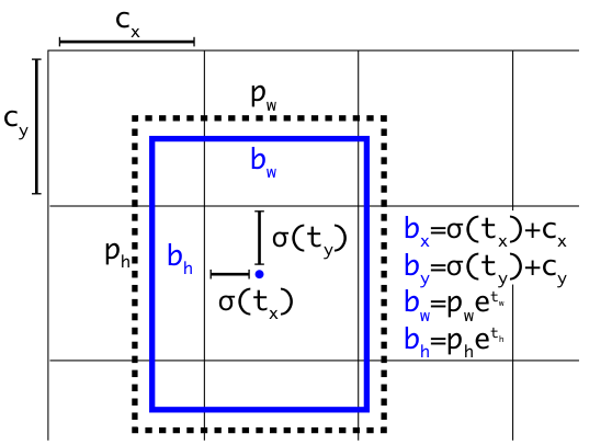
The code for this is shown below:
        bbox_xywh = xywh_energy.clone().detach()

        # Cell offsets C_x and C_y from original paper.
        cx = torch.linspace(0, w - 1, w, device=self.device).repeat(h, 1)
        cy = torch.linspace(
            0, h - 1, h, device=self.device
        ).repeat(w, 1).t().contiguous()

        # Get bbox center x and y coordinates.
        bbox_xywh[:, :, 0, :, :].sigmoid_().add_(cx).div_(w)
        bbox_xywh[:, :, 1, :, :].sigmoid_().add_(cy).div_(h)

        # Anchor priors (P_w and P_h in original paper).
        anchors = self.anchors

        anchor_w = torch.tensor(
            anchors, device=self.device
        )[:, 0].reshape(1, num_anchors, 1, 1)

        anchor_h = torch.tensor(
            anchors, device=self.device
        )[:, 1].reshape(1, num_anchors, 1, 1)

        # Get bbox width and height.
        bbox_xywh[:, :, 2, :, :].exp_().mul_(anchor_w)
        bbox_xywh[:, :, 3, :, :].exp_().mul_(anchor_h)
The objectness score (probability that the bounding box actually contains an object) is obtained from the objectness energy by applying the sigmoid function. The class energies are converted to class scores (likelihood that the object belongs to each respective class) by applying the softmax function to the class energies. The actual class probabilities are obtained by multiplying the class scores with the objectness score. Because there are three YOLO layers, it's convenient to be able to combine the detections from all three YOLO layers at the end of the forward pass in Darknet.forward(); thus, the bounding box coordinates and the bounding box probability and class index tensors (corresponding to the class with the greatest probability for each bounding box) are reshaped such that they can be concatenated:
|
|
Here, we're permuting the indices of the bounding box coordinate tensor
bbox_xywh —a tensor of shape \([B, A, 4, H, W]\) (where the four
coordinates are center x, center y, width, and height) for each of W*H grid
cells—to a tensor of shape \([B, A, H, W, 4]\), i.e., placing the anchor
index and grid cell indices in the middle and the coordinate index at the end.
Then, we reshape this by combining the grid cells for each anchor box scale via
reshape(batch_size, -1, 4) into a tensor of shape \([B, (A \times H \times W),
4]\). This allows us to easily concatenate this tensor of detections with those
from other YOLO layers along the middle (detection) index. We perform a similar
operation for the class probability and class index tensors.
Combining output from multiple YOLO layers
Now we arrive at the Darknet.forward() method, which receives its input from the inference function introduced earlier. First, we initialize a dictionary to store the outputs from the shortcut and route layers that need to be cached. Then we initialize empty lists that will store the outputs from each YOLO layer.
    def forward(self, x):
        """
        Returns:
            Dict of bbox coordinates, class probabilities and class indices.
        """
        # Outputs from layers to cache for shortcut/route connections.
        cached_outputs = {
            block_idx: None for block_idx in self.blocks_to_cache
        }

        # Lists of transformed outputs from each YOLO layer to be concatenated.
        bbox_xywh_list = []
        class_prob_list = []
        class_idx_list = []
Next, we iterate through each block and call the forward method of the
appropriate module from self.modules_ (if it's a convolutional, maxpool, or
upsample block), sum/concatenate the current layer with the appropriate cached
layers (if it's a route or shortcut block), or append the YOLO layer output to
the aforementioned lists (if it's a yolo block).
        for i, block in enumerate(self.blocks):
            if block["type"] in ("convolutional", "maxpool", "upsample"):
                x = self.modules_[i](x)
            elif block["type"] == "route":
                # Concatenate outputs from layers specified by the "layers"
                # field of the route block.
                x = torch.cat(
                    tuple(cached_outputs[idx] for idx in block["layers"]),
                    dim=1
                )
            elif block["type"] == "shortcut":
                # Add output from previous layer with the output from the layer
                # specified by the "from" field of the shortcut block.
                x = cached_outputs[i-1] + cached_outputs[i+block["from"]]
            elif block["type"] == "yolo":
                bbox_xywh, class_prob, class_idx = self.modules_[i](x)
                bbox_xywh_list.append(bbox_xywh)
                class_prob_list.append(class_prob)
                class_idx_list.append(class_idx)

            if i in cached_outputs:
                cached_outputs[i] = x
Finally, we call torch.cat() on the lists of YOLO outputs to concatenate them.
Unlike YOLOv2 (which predicted bounding box width and height as fractions of
image dimensions), the YOLO layers in YOLOv3 return bounding box width and
height in absolute pixel values based on the width and height of the images on
which the network was trained. This information is contained in the model .cfg
file and was
extracted by the parse_config() function
discussed in the last post.
Therefore, we need to scale these values accordingly. The resulting bounding box
width and height values give us the bounding box dimensions relative to image
dimensions (in other words, a height of 0.14 for a given detection in
bbox_xywh, e.g., bbox_xywh[0, 0, 3], would tell us that the height of this
bounding box is 14% of the input image height).
        # Concatenate predictions from each scale (ie, each YOLO layer).
        bbox_xywh = torch.cat(bbox_xywh_list, dim=1)
        class_prob = torch.cat(class_prob_list, dim=1)
        class_idx = torch.cat(class_idx_list, dim=1)

        # Scale bbox w and h based on training width/height from net info.
        train_wh = torch.tensor(
            [self.net_info["width"], self.net_info["height"]],
            device=self.device
        )
        bbox_xywh[:, :, 2:4].div_(train_wh)

        return {
            "bbox_xywh": bbox_xywh,
            "class_prob": class_prob,
            "class_idx": class_idx,
        }
Post-processing
Let's return to inference.inference(), where we perform some post-processing on the output of Darknet.forward().
    out = net.forward(inp)

    bbox_xywh = out["bbox_xywh"].detach().cpu().numpy()
    class_prob = out["class_prob"].cpu().numpy()
    class_idx = out["class_idx"].cpu().numpy()

    thresh_mask = class_prob >= prob_thresh
The output of the network is first converted from PyTorch tensors to numpy arrays, after which we create a boolean mask to isolate only the detections exceeding the specified probability threshold.
    # Perform post-processing on each image in the batch and return results.
    results = []
    for i in range(bbox_xywh.shape[0]):
        image_bbox_xywh = bbox_xywh[i, thresh_mask[i, :], :]
        image_class_prob = class_prob[i, thresh_mask[i, :]]
        image_class_idx = class_idx[i, thresh_mask[i, :]]

        image_bbox_xywh[:, [0, 2]] *= orig_image_shapes[i][1]
        image_bbox_xywh[:, [1, 3]] *= orig_image_shapes[i][0]
        image_bbox_tlbr = cxywh_to_tlbr(image_bbox_xywh.astype(np.int))

        idxs_to_keep = non_max_suppression(
            image_bbox_tlbr, image_class_prob, class_idx=image_class_idx,
            iou_thresh=nms_iou_thresh
        )

        results.append(
            [
                image_bbox_tlbr[idxs_to_keep, :],
                image_class_prob[idxs_to_keep],
                image_class_idx[idxs_to_keep]
            ]
        )

    return results
Next, we iterate over each image in the batch. The bounding box coordinates are
scaled based on the original (unresized) dimensions of the image. For
convenience, we convert the bounding box coordinates from "cxywh" (center x,
center y, width, height) to "tlbr" (top left x, top left y, bottom right x,
bottom right y). Finally, there's non-maximum suppression (NMS), which is
arguably the most important step in which we remove duplicate detections. I
won't get into the implementation of NMS I've used here (maybe I'll cover it in
a future post), but the highlights are that 1) we perform per-class NMS, meaning
that each class is treated separately (so there might end up being bounding
boxes for different classes that overlap) and 2) of any bounding boxes that
sufficiently overlap each other (where "sufficient" is defined as having an
intersection over union greater than or equal to nms_iou_thresh), only the
one with the highest probability is kept.
The thresholding and NMS steps are demonstrated in the animation below:
The first frame shows all bounding boxes. The second frame shows all bounding boxes after a nominal probability threshold has been applied. The last frame shows the bounding boxes remaining after NMS. Each class is represented with a distinct color. Because we perform per-class NMS, bounding boxes of different classes may significantly intersect one another.
In the end, we're left with results, a list of lists where each inner list
contains bounding box data for an image from the batch.
Summary
These first few posts have examined the process of constructing the network, preprocessing the input images, pushing data through the network, and postprocessing the network output to extract actual detections and bounding boxes (i.e., defining/instantiating the network and performing inference). In the next post, we'll build upon this to run the framework on images and video in real time.