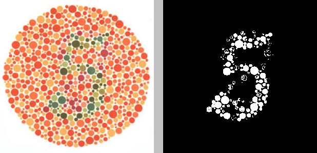
If you’re sighted and have ever been to an eye doctor, you’ve probably seen an Ishihara color blindness test—you know, the tests with the patterns of colored bubbles that contain a number in the middle:

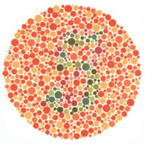
People with normal vision should be able to see the number “5” in this image. On the other hand, if you’re like me and have mild red-green color blindness, it might just look like a jumble of red and orange dots with an indistinct smattering of green dots in the middle. Individuals who are red-green color blind have trouble distinguishing shades of red from shades of green. Less common is blue-yellow color blindness and least common is total color blindness. In the image above, most of the dots are shades of red, with the number 5 formed by dots that are shades of green. Since the red-green color blind have trouble telling these hues apart, they may find it difficult or impossible to make out the number 5.

K-means clustering is a machine learning technique used to separate data into distinct groups. Although I won’t go into the details of how the K-means clustering algorithm works, you can find plenty of resources online that explain it, and the first and second posts of this blog focus on animating the algorithm to give you an idea of how to visualize it.

Image segmentation refers to splitting an image into different parts, depending on how we wish to analyze it. For example, if we were trying to track a ball in a video and wanted to isolate the ball, we might segment the image using edge detection to find round objects and filter out everything else. In this case, we’d like to group the pixels in images of color blindness tests such that the relevant parts of the image (the numbers) are in one cluster, and everything else is in some other cluster. We’re going to apply K-means clustering to separate the number in an Ishihara color blindness test from the background.

Colors and clustering

Colors in digital images are most frequently represented by the RGB color model, which describes color in terms of the amount of red, blue, and green it contains. In an 8-bit representation, where numbers can take on a value from 0 to 255, (0, 0, 0) represents black, i.e., none of each color, and (255, 255, 255) represents white, i.e., the maximum amount of each color. A light shade of blue might be represented by (0, 0, 255), and a dark shade of blue by (0, 0, 80).

Before performing K-means clustering on the previous image, we must first determine how many clusters (the “K” in “K-means”) to group the pixels into. We might decide on three clusters, since there are three major colors in the image—the white background, the red/orange dots that form the circle, and the green dots that form the number. Finally, since each color is represented by three values (RGB), we might decide to apply the K-means algorithm in three dimensions, which refers to the fact that we’re grouping pixels into one of three clusters based on the frequency with which all three values (RGB) occur together in all the pixels. The result looks like this:

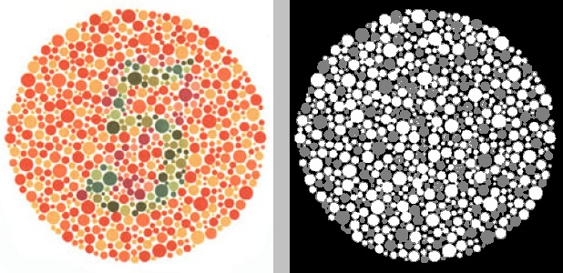
On the left is the original image. The grayscale image on the right represents the K-means clustering of the original image. Each shade in the image on the right (white, gray, black) represents one cluster. Although the background (white in the original image, black in the K-means image) has been properly grouped into its own cluster, the red and green dots from the original have not been; in the K-means image, they form an indistinct mix of white and gray dots. That’s because, per the RGB model, all the colored dots contain varying amounts of red, green, and blue. The red/orange dots might contain more red and the green dots might contain more green, but the differences are not clear enough (especially when taking into account blue) for the K-means algorithm to properly distinguish them.

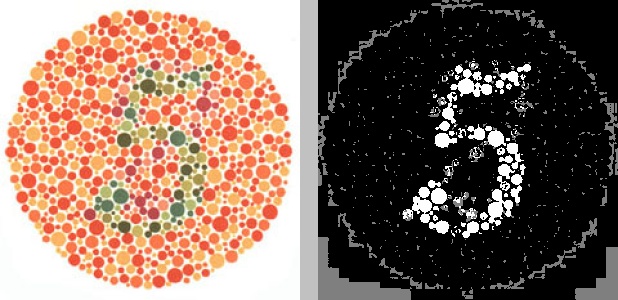
OK, so what if we instead perform K-means clustering on just one of the three RGB channels—green? In other words, if we ignore the red and blue channels and split the pixels into three groups based on how much green they contain, we might expect to see three distinct groups emerge: 1) the white background, which contains the maximum intensity of green, 2) the green dots that form the number 5, and 3) the red dots, which contain the least green. This is what it looks like:

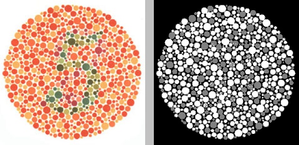
Unfortunately, this is just as unhelpful as the last attempt. Because there are so many red-orange dots of different hues, which contain varying amounts of green, and so many different green dots that are different intensities of green, K-means applied to the green channel doesn’t help.

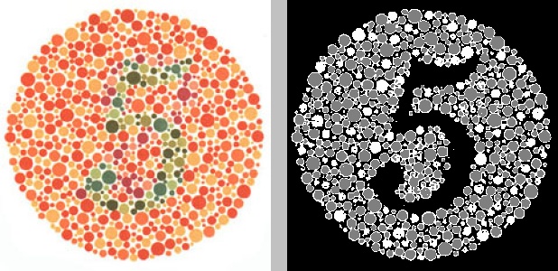
What if we try the same thing but with the red channel? This is the result:

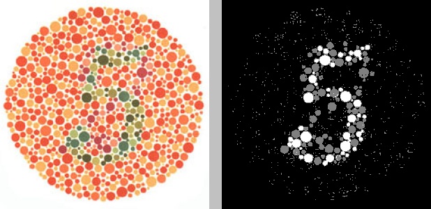
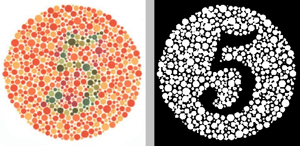
This is better! We finally see the 5 emerge (or is it an 8?), though there’s still a fair bit of noise. What if, instead of three clusters, we grouped the red channel into two clusters, so everything in one cluster was white and everything in the other cluster was black, based on how much red it contained in the original image?

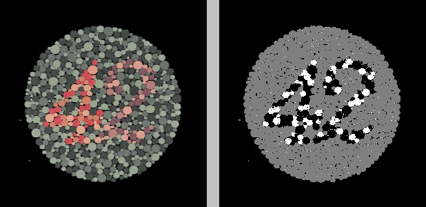
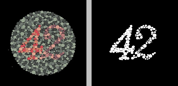
Much cleaner, though there’s still a bit of noise. And, of course, it took us several tries, tweaking the parameters of the algorithm (number of clusters and number of channels), to arrive at this. What happens if we apply the same parameters—two clusters, red channel only—to a different Ishihara test?

Looks like these parameters fail on the new image, which contains a two-digit number, 42, in a circle of green dots. One digit of the number, the 4, is a more intense shade of red, while the other digit, the 2, is a drab shade of red that’s considerably more similar to its surrounding green dots. Neither can be clearly discerned in the clustered image.

By the way, if you’re wondering how the color for each cluster was chosen in the grayscale images, it’s based on the number of pixels that belong to each cluster. The cluster containing the most pixels is assigned black and the cluster containing the fewest pixels is assigned white (from which you can guess how the shades of gray are selected, for cases with more than two clusters).

The HSV color space

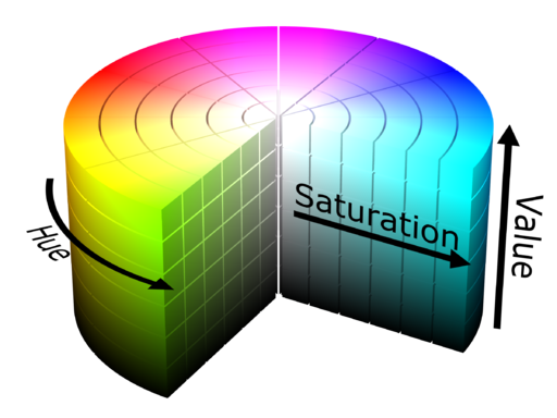
One issue with the RGB color model is that it requires three values to specify any given hue. What if, instead, we could specify hue with a single value? This might facilitate clustering using K-means, since we wouldn’t have to worry about how often three particular values occur simultaneously. Furthermore, it might avoid the issue of having to determine which channel to use, as we did above. Enter the HSV color model, whose three channels represent the hue, saturation, and intensity value, respectively, of a color. This can be visualized with a cylinder (image borrowed from Wikimedia Commons):

Since different hues are represented by distinct values along a (cylindrical) spectrum, it should theoretically be easier to group distinct colors into distinct clusters, assuming they are sufficiently different from one another. If we convert our original image of the number 5 into its HSV representation, then apply K-means clustering on the hue channel with three clusters, we get the following:

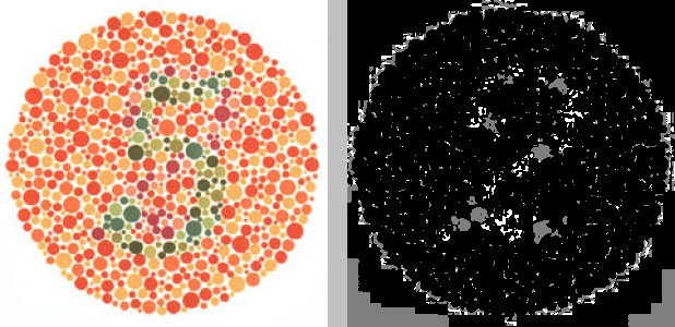
Not only has the white background been clustered with many of the colored dots, but the number 5 is not visible at all. Instead, a hidden, muddled number 2 has appeared. Because the hue channel of the HSV representation of an image doesn’t account for brightness or contrast, we might try performing two-dimensional K-means clustering on the image using both the hue and value channels instead of just the hue channel:

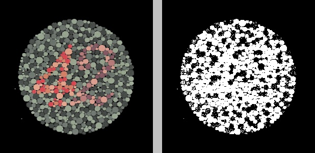
Better, though still somewhat messy. What if we convert the other image, which contains the number 42, to the HSV color space and then apply K-means clustering on just the hue channel?

The number 42 is clearly visible, though it seems to be split between two clusters. I’ll spare you the result of applying K-means clustering on both the hue and value channels simultaneously, in which the number cannot be clearly identified.

The Lab color space

The RGB color model uses three values to specify hue and the HSV color model uses one value to specify hue, while the Lab color model utilizes two values to specify hue. The “L” in Lab refers to the lightness of the color, the “a” represents the red-green component, and the “b” represents the blue-yellow component. In other words, a red color will have a large value for “a”, whereas a green color will possess a small value for “a”. This makes it perfect for clustering the colors in a typical Ishihara test. Here is the result of converting the image to its Lab representation and running K-means clustering with three clusters on just the “a” channel:

There’s no doubt about the number 5 in this image. Applying K-means clustering with just two clusters to the “a” channel of the Lab representation of the number 42 works, perhaps, even better:

The YCbCr color space

There exist literally dozens of color spaces, and it would be impractical to go through them all, but I will briefly mention one more: the YCbCr color space, sometimes also abbreviated YCC. The YCbCr model represents color using a “Y” component (luma), a “Cb” component (blue-difference), and a “Cr” component (red-difference). Note that, if you’re using OpenCV, these last two components are swapped—OpenCV puts them in the order “YCrCb”. The YCbCr color model is fundamentally similar to the Lab color space in that its blue-difference component “Cb” contains blue on one end of its spectrum and yellow on the other end, much like the Lab model’s “b” component, and the red-difference component “Cr” contains red on one end of its spectrum and green on the other, like the Lab model’s “a” component. Thus, you might expect that applying K-means clustering to the “Cr” channel of the YCC representation of an image would produce results similar to those for the Lab cases above. You would be right:

In both of the above examples, the pixels have only been grouped into two clusters.

Comparing clustering between the different color spaces

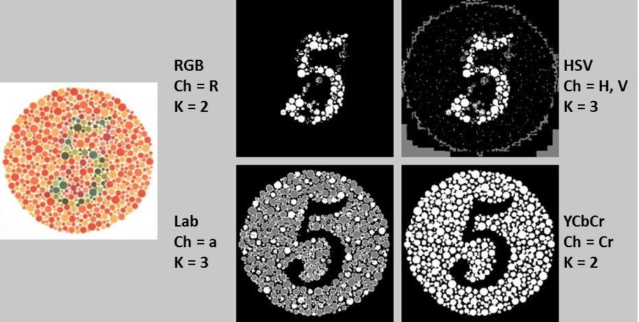
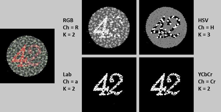
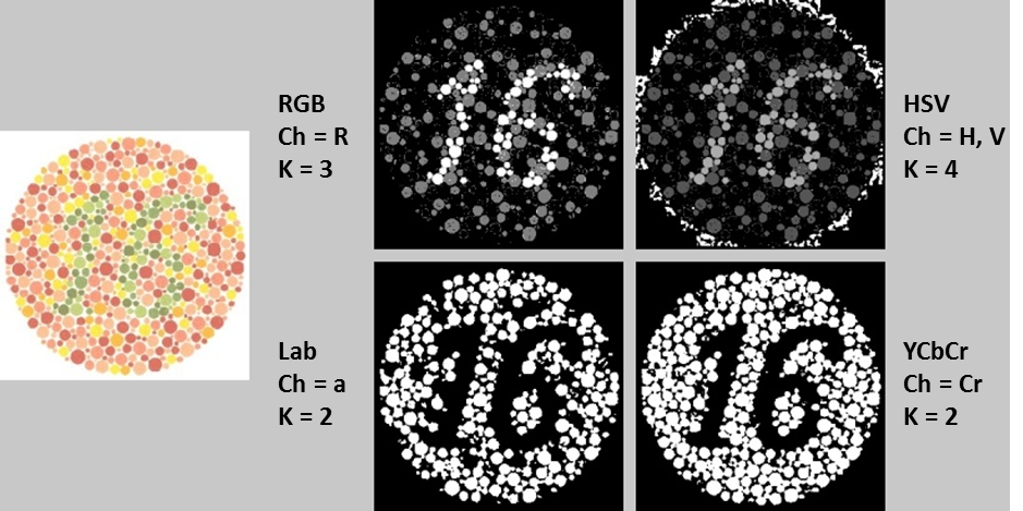
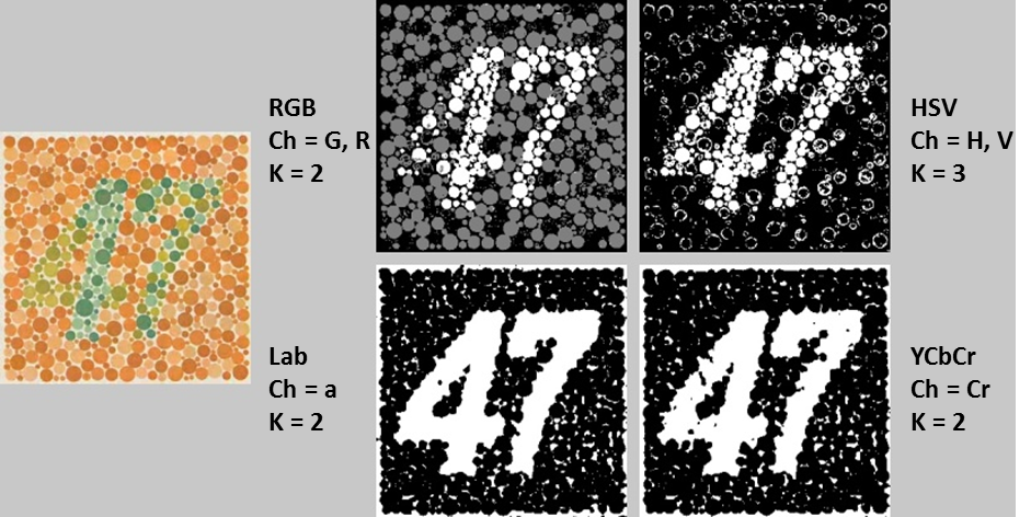
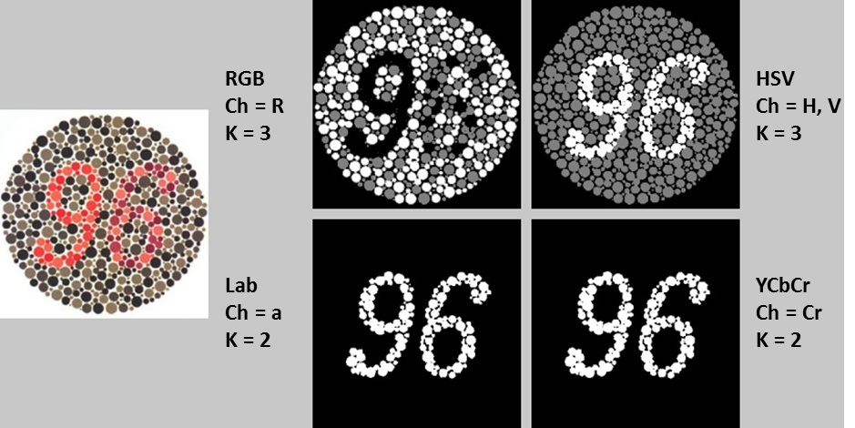
I’ll end this post with a handful of additional Ishihara tests and their clustered counterparts using the color spaces discussed above. In each case, I tuned the parameters to obtain the optimal (read: most readable) result. It should be noted that performing K-means clustering on the Lab and YCbCr representations tended to yield the most clear and consistent results, generally requiring only two clusters and one channel. The original images are on the left, and their grayscale K-means counterparts are on the right. Beside each K-means image is a text label indicating 1) the color space used for analysis, 2) the channel(s) from the color space on which K-means clustering was performed, and 3) the number of clusters “K” into which the image pixels were grouped.

Hopefully, this post has given you an idea of when, why, and how it might be useful to use different color spaces for image segmentation.