
The previous post discussed the use of K-means clustering and different color spaces to isolate the numbers in Ishihara color blindness tests:
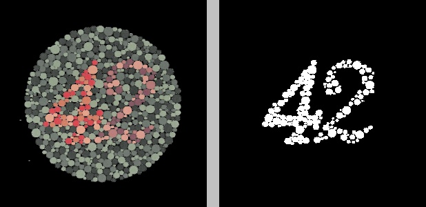
In the figure above, the original image on the left was converted to the YCrCb color space, after which K-means clustering was applied to the Cr channel to group the pixels into two clusters. The result is the image on the right, where black represents one cluster and white represents the other cluster.
In this post, we’ll go through the Python code that produced this figure (and the other figures from the previous post) using OpenCV and scikit-learn.
The code
The
script can be found on my github, if you’re so inclined. Otherwise,
fire up a text editor and create a file named color_segmentation.py.
|
|
First, the necessary imports. The datetime module will be used to construct a
unique timestamped filename for the output image.
|
|
Next, we construct the argument parser to handle input options and parameters. The usage of each flag can be seen from its respective help text above and should also become more clear as we go through the rest of the code.
|
|
Line 25 puts the input arguments into a dictionary args. Line 26 reads
the input image and stores it in image. If a width was specified by the user,
lines 29-32 resize the image using the OpenCV function resize(). At this
stage, we create a copy of the image on line 33 since we’ll continue
to modify the image (this allows us to use or display the original later).
|
|
Next, the image is converted to the desired color space, if the user specified
one, using OpenCV’s cvtColor() function. Note that OpenCV utilizes the
BGR color space by default, not RGB, when it reads in an image with
cv2.imread() or displays a color image with cv2.imshow().
|
|
Now that the image has been converted to the correct color space, we’ll
isolate only the channels on which we wish to perform K-means clustering. The
channels input argument takes a string of digits, where each digit represents
a channel index. For example, in the BGR color space, channel 0 would be B (the
blue channel), 1 would be G (the green channel), and 2 would be R (the red
channel). Similarly, if we’d converted the image to the YCrCb color space,
0 would denote channel Y (luma), 1 would denote channel Cr (red-difference), and
2 would denote channel Cb (blue-difference). For example, a user input of
“01” would mean we wish to use channels 0 and 1 for K-means
clustering. An input of “2” would mean we wish to use only channel 2
for K-means clustering. If only a single channel is selected, the resulting
numpy array loses its third dimension (an image array’s first index
represents the row, its second index represents the column, and the third index
represents the channel). Lines 53-54 check for this and simply
“reshape” the array by adding a dummy third index of length 1, if
necessary, so the array works with the upcoming code.
|
|
The scikit-learn K-means clustering method KMeans.fit() takes a 2D array whose
first index contains the samples and whose second index contains the features
for each sample. In other words, each row in the input array to this function
represents a pixel and each column represents a channel. We achieve this by
reshaping the image array on line 58. Lines 61-62 ensure that a value of
at least 2 clusters was chosen (since classifying the pixels into a single
cluster would be meaningless).
Line 64 actually applies K-means clustering to the input array.
KMeans(n_clusters=numClusters, n_init=40, max_iter=500) creates a KMeans
object with the given parameters. n_init=40 means that K-means clustering will
be run 40 times on the data, with the initial centroids randomized to different
locations each time, from which the best result will be returned. 40 isn’t some
universal magic number—I simply tried a few different values and found it
to be the lowest value that provided consistent results. max_iter=500 means
that, during each of those 40 runs, the cluster centroids will be updated until
they stop changing or until the algorithm has continued for 500 iterations.
Again, 500 isn’t a magic number. I simply found it to provide the most
consistent results. fit(reshaped) actually runs the algorithm using these
parameters on our dataset.
|
|
After running the K-means clustering algorithm, we retrieve the cluster labels
using the labels_ member array of the KMeans object. We reshape this back
into the image’s original 2D shape on lines 68-69.
Since we’re going to display the clustered result as a grayscale image, it makes
sense to assign hues (black, white, and as many shades of gray in between as are
necessary) to the clusters in a logical order. The cluster labels won’t
necessarily be the same each time K-means clustering is performed, even if the
pixels in the image are grouped into the same clusters—e.g.,
KMeans.fit() might, on one run, put the pixels of the number in a color
blindness test into cluster label “0” and the background pixels into cluster
label “1”, but running it again might group pixels from the number into cluster
label “1” and the background pixels into cluster label “0”. However, assuming
the pixels are clustered the same way each time (even if the clusters end up
with different labels), the total number of pixels in any given cluster
shouldn’t change between runs. Lines 72-73 exploit this by putting the
cluster labels in a list sorted by the frequency with which they occur in the
clustered image, from most to least frequent.
|
|
Finally, we create a single-channel 8-bit grayscale image where each pixel is
assigned a hue based on the cluster to which it belongs and the frequency of the
cluster (from the sorted list of labels). In an 8-bit grayscale image, a pixel
with a value of 0 is black and a pixel with a value of 255 is white, which is
where 255 comes from on line 78. At this point, we could stop and display
the grayscale image with a call to cv2.imshow(). For convenience, though,
let’s put the original image and the resulting clustered image, kmeansImage,
side by side:
|
|
Since we want to show the original BGR image alongside the clustered grayscale
image, we have to convert the grayscale image to BGR. For clarity, I’ve opted to
add a strip of gray between the two images, whose hue is given by the arbitrary
value 193, whose height is the same as that of the images, and whose width I’ve
defined as a percentage (6.25%) of the image width. The original image, gray
divider, and clustered image are stacked horizontally with a call to the numpy
function concatenate().
|
|
Lastly, if the user supplied the --output-file option, lines 86-93
construct a timestamped filename that contains the name of the chosen color
space, the channel indices, and the number of clusters used for clustering, then
write the image to disk with a call to cv2.imwrite(). Line 94 waits until
any key is pressed to close the window previously displayed by cv2.imshow().
Usage
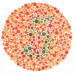
Say we had the following source image, named ishihara_5_original.jpg:
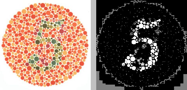
We might run the following in our terminal or command line window:
python color_segmentation.py -i ishihara_5_original.jpg -w 300 -s hsv -c 02 -n 3 -o -f jpgThis translates to “resize the source image ishihara_5_original.jpg
(-i ishihara_5_original.jpg) to a width of 300 pixels (-w 300), convert it
to the HSV color space (-s hsv), then perform K-means clustering on channels 0
and 2 (-c 02) by grouping the pixels into 3 clusters (-n 3) and output the
resulting file (-o) in JPG format (-f jpg). " The result would look like
this:
The resulting filename of the output image would be something like
2018329194036hsv_c02n3.jpg. Recall from the beginning of the file that all
arguments except the source image filename are optional, though the defaults
won’t necessarily provide optimal clustering. For example, this is what happens
if we just run it with the default settings—BGR color space (equivalent to
specifying the option -s bgr), all channels (equivalent to specifying -c 012
or -c all), and 3 clusters:
python color_segmentation.py -i ishihara_5_original.jpg -w 300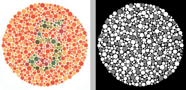
Try the script on your own images, or tweak it to your liking.